On the night of February 21, 2003 a physician from Guangdong Province in southern China checked into the Metropole Hotel in Hong Kong. He previously treated patients suffering from a disease that, lacking a clear diagnosis, was called atypical pneumonia. Next day, after leaving the hotel, he went to the local hospital, this time as a patient. He died there several days later of atypical pneumonia [1].
The physician did not leave the hotel without a trace: That night sixteen other guests of the Metropole Hotel and one visitor also contracted the disease that was eventually renamed Severe Acute Respiratory Syndrome, or SARS. These guests carried the SARS virus with them to Hanoi, Singapore, and Toronto, sparking outbreaks in each of those cities. Epidemiologists later traced close to half of the 8,100 documented cases of SARS back to the Metropole Hotel. With that the physician who brought the virus to Hong Kong become an example of a super-spreader, an individual who is responsible for a disproportionate number of infections during an epidemic.
A network theorist will recognize super-spreaders as hubs, nodes with an exceptional number of links in the contact network on which a disease spreads. As hubs appear in many networks, super-spreaders have been documented in many infectious diseases, from smallpox to AIDS [2]. In this chapter we introduce a network based approach to epidemic phenomena that allows us to understand and predict the true impact of these hubs. The resulting framework, that we call network epidemics, offers an analytical and numerical platform to quantify and forecast the spread of infectious diseases.
Image 10.1
Super-spreaders
One-hundred-forty-four of the 206 SARS patients diagnosed in Singapore were traced to a chain of five individuals that included four super-spreaders. The most important of these was Patient Zero, the physician from Guangdong Province in China, who brought the disease to the Metropole Hotel. After [1].
Infectious diseases account for 43% of the global burden of disease, as captured by the number of years of lost healthy life. They are called contagious, as they are transmitted by contact with an ill person or with their secretions. Cures and vaccines are rarely sufficient to stop an infectious disease - it is equally important to understand how the pathogen responsible for the disease spreads in the population, which in turn determines the way we administer the available cures or vaccines.
The diversity of phenomena regularly described as spreading processes on networks is staggering:
Biological
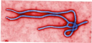
The spread of pathogens on their respective contact network is the main subject of this chapter. Examples include airborne diseases like influenza, SARS, or tuberculosis, transmitted when two individuals breathe the air in the same room; contagious diseases and parasites transmitted when people touch each other; the Ebola virus, transmitted via contact with a patient's bodily fluids, HIV and other sexually transmitted diseases passed on during sexual intercourse. Infectious diseases also include cancers carried by cancer-causing viruses, like HPV or EBV, or diseases carried by parasites like bedbugs or malaria.
Digital
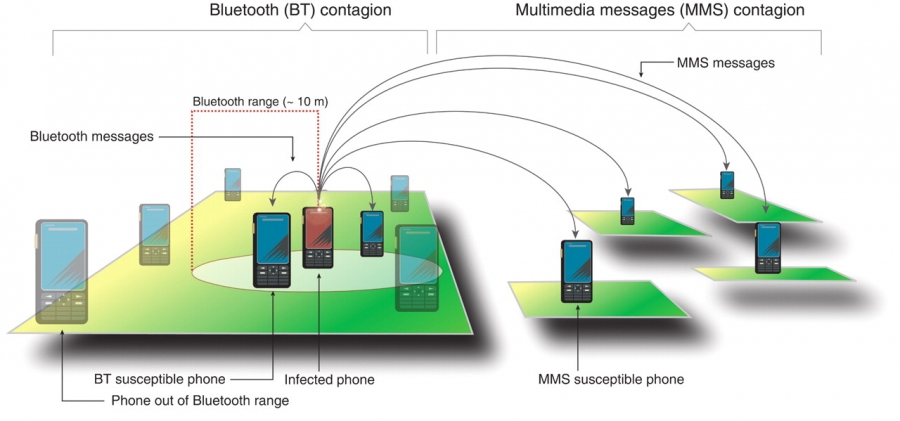
A computer virus is a self-reproducing program that can transmit a copy of itself from computer to computer. Its spreading pattern has many similarities to the spread of pathogens. But digital viruses also have many unique features, determined by the technology behind the specific virus. As mobile phones morphed into hand-held computers, lately we also witnessed the appearance of mobile viruses and worms that infect smartphones (Image 10.2).
Image 10.2
Mobile Phone Viruses
Smart phones, capable of sharing programs and data with each other, offer a fertile ground for virus writers. Indeed, since 2004 hundreds of smart phone viruses have been identified, reaching a state of sophistication in a few years that took computer viruses about two decades to achieve [3]. Mobile viruses are transmitted using two main communication mechanisms [4]:
Bluetooth (BT) Viruses
A BT virus infects all phones found within BT range from the infected phone, which is about 10-30 meters. As physical proximity is essential for a BT connection, the transmission of a BT virus is determined by the owner’s location and the underlying mobility network, connecting locations by individuals who travel between them (SECTION 10.4). Hence BT viruses follow a spreading pattern similar to influenza.
Multimedia Messaging Services (MMS)
Viruses carried by MMS can infect all susceptible phones whose number is in the infected phone’s phonebook. Hence MMS viruses spread on the social network, following a long-range spreading pattern that is independent of the infected phone’s physical location. Consequently the spreading of MMS viruses is similar to the patterns characterizing computer viruses.
Social
The role of the social and professional network in the spread and acceptance of innovations, knowledge, business practices, products, behavior, rumors and memes, is a much-studied problem in social sciences, marketing and economics [5, 6]. Online environments, like Twitter, offer unprecedented ability to track such phenomena. Consequently a staggering number of studies focus on social spreading, asking for example why can some messages reach millions of individuals, while others struggle to get noticed.
The examples discussed above involve diverse spreading agents, from biological to computer viruses, ideas and products; they spread on different types of networks, from social to computer and professional networks; they are characterized by widely different time scales and follow different mechanisms of transmission (Table 10.1). Despite this diversity, as we show in this chapter, these spreading processes obey common patterns and can be described using the same network-based theoretical and modeling framework.
Phenomena
Agent
Network
Venereal Disease
Pathogens
Sexual Network
Rumor Spreading
Information, Memes
Communication Network
Diffusion of Innovations
Ideas, Knowledge
Communication Network
Computer Viruses
Malwares, Digital viruses
Internet
Mobile Phone Virus
Mobile Viruses
Social Network/Proximity Network
Bedbugs
Parasitic Insects
Hotel - Traveler Network
Malaria
Plasmodium
Mosquito - Human network
Table 10.1
Networks and Agents
The spread of a pathogen, a meme or a computer virus is determined by the network on which the agent spreads and the transmission mechanism of the responsible agent. The table lists several much studied spreading phenomena, together with the nature of the particular spreading agent and the network on which the agent spreads.
Section 10.2
Epidemic Modeling
Epidemiology has developed a robust analytical and numerical framework to model the spread of pathogens. This framework relies on two fundamental hypotheses:
Compartmentalization
Epidemic models classify each individual based on the stage of the disease affecting them. The simplest classification assumes that an individual can be in one of three states or compartments:
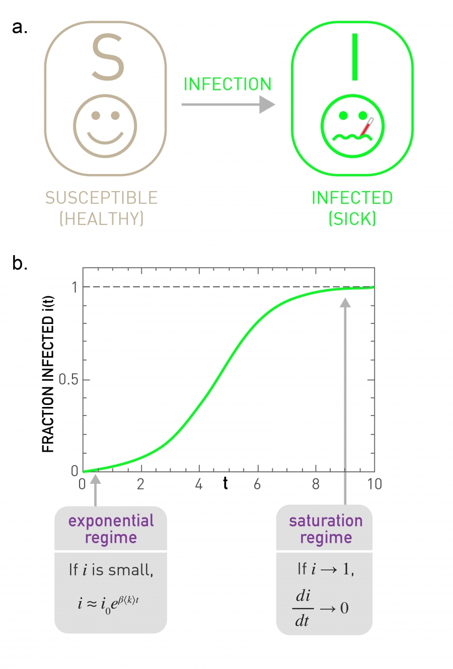
Susceptible (S): Healthy individuals who have not yet contacted the pathogen (Image 10.3).
Infectious (I): Contagious individuals who have contacted the pathogen and hence can infect others.
Recovered (R): Individuals who have been infected before, but have recovered from the disease, hence are not infectious.
The modeling of some diseases requires additional states, like immune individuals, who cannot be infected, or latent individuals, who have been exposed to the disease, but are not yet contagious.
Individuals can move between compartments. For example, at the beginning of a new influenza outbreak everyone is in the susceptible state. Once an individual comes into contact with an infected person, she can become infected. Eventually she will recover and develop immunity, losing her susceptibility to the the particular strain of influenza.
Homogenous Mixing
The homogenous mixing hypothesis (also called fully mixed or mass-action approximation) assumes that each individual has the same chance of coming into contact with an infected individual. This hypothesis eliminates the need to know the precise contact network on which the disease spreads, replacing it with the assumption that anyone can infect anyone else.
Image 10.3
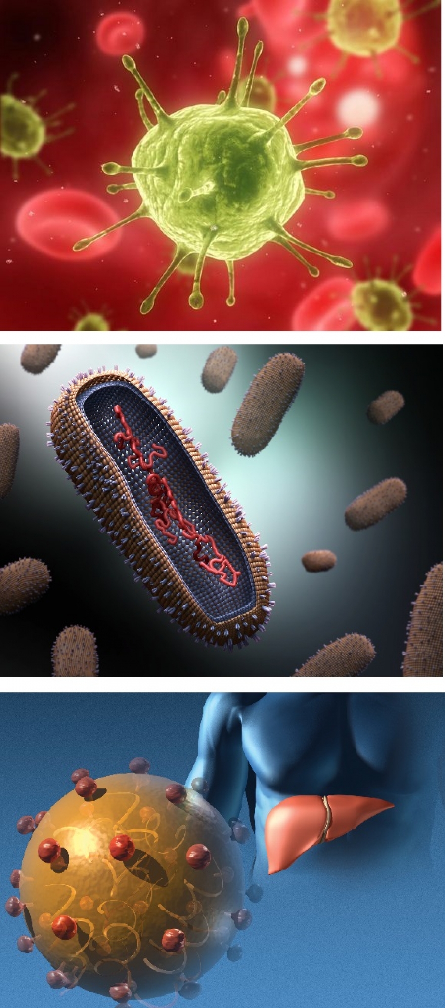
Pathogens
A pathogen, a word rooted in the Greek words “suffering, passion” (pathos) and “producer of” (genes), denotes an infectious agent or germ. A pathogen could be a disease-causing microorganism, like a virus, a bacterium, a prion, or a fungus. The figure shows several much-studied pathogens, like the HIV virus, responsible for AIDS, an influenza virus and the hepatitis C virus. After http://www.livescience.com/18107-hiv-therapeutic-vaccines-promise.html and http://www.huffingtonpost.com/2014/01/13/deadly-viruses-beautiful-photos_n_4545309.html
In this section we introduce the epidemic modeling framework built on these two hypotheses. To be specific, we explore the dynamics of three frequently used epidemic models, the so-called SI, SIS and SIR models, that help us understand the basic building blocks of epidemic modeling.
Susceptible-Infected (SI) Model
Consider a disease that spreads in a population of N individuals. Denote with S(t) the number of individuals who are susceptible (healthy) at time t and with I(t) the number individuals that have been already infected. At time t=0 everyone is susceptible (S(0)=N) and no one is infected (I(0)=0). Let us assume that a typical individual has 〈k〉 contacts and that the likelihood that the disease will be transmitted from an infected to a susceptible individual in a unit time is β. We ask the following: If a single individual becomes infected at time t=0 (i.e. I(0)=1), how many individuals will be infected at some later time t?
Within the homogenous mixing hypothesis the probability that the infected person encounters a susceptible individual is S(t)/N. Therefore the infected person comes into contact with 〈k〉S(t)/N susceptible individuals in a unit time. Since I(t) infected individuals are transmitting the pathogen, each at rate β, the average number of new infections dI(t) during a timeframe dt is
Consequently I(t) changes at the rate
Throughout this chapter we will use the variables
to capture the fraction of the susceptible and of the infected population at time t. For simplicity we also drop the (t) variable from i(t) and s(t), re-writing (10.1) as (ADVANCED TOPICS 10.A)
where the product β〈k〉 is called the transmission rate or transmissibility. We solve (10.3) by writing
Integrating both sides, we obtain
With the initial condition i0= i(t=0), we get C=i0/(1–i0), obtaining that the fraction of infected individuals increases in time as
Equation (10.4) predicts that:
At the beginning the fraction of infected individuals increases exponentially (Image 10.4b). Indeed, early on an infected individual encounters only susceptible individuals, hence the pathogen can easily spread.
The characteristic time required to reach an 1/e fraction (about 36%) of all susceptible individuals is
Hence τ is the inverse of the speed with which the pathogen spreads through the population. Equation (10.5) predicts that increasing either the density of links〈k〉 or β enhances the speed of the pathogen and reduces the characteristic time.
With time an infected individual encounters fewer and fewer susceptible individuals. Hence the growth of i slows for large t (Image 10.4b). The epidemic ends when everyone has been infected, i.e. when i(t→∞)=1 and s(t→∞)=0.
Image 10.4
The Susceptible-Infected (SI) Model
In the SI model an individual can be in one of two states: susceptible (healthy) or infected (sick). The model assumes that if a susceptible individual comes into contact with an infected individual, it becomes infected at rate β. The arrow indicates that once an individual becomes infected, it stays infected, hence it cannot recover.
Time evolution of the fraction of infected individuals, as predicted by (10.4). At early times the fraction of infected individuals grows exponentially. As eventually everyone becomes infected, at large times we have i(∞)=1.
Susceptible-Infected-Susceptible (SIS) Model
Most pathogens are eventually defeated by the immune system or by treatment. To capture this fact we need to allow the infected individuals to recover, ceasing to spread the disease. With that we arrive at the so-called SIS model, which has the same two states as the SI model, susceptible and infected. The difference is that now infected individuals recover at a fixed rate μ, becoming susceptible again (Image 10.5a). The equation describing the dynamics of this model is an extension of (10.3),
where μ is the recovery rate and the μi term captures the rate at which the population recovers from the disease. The solution of (10.6) provides the fraction of infected individuals in function of time (Image 10.5b)
where the initial condition i0=i(t=0) gives C=i0/(1–i0 –µ/β〈k〉).
Image 10.5
The Susceptible-Infected-Susceptible (SIS) Model
The SIS model has the same states as the SI model: susceptible and infected. It differs from the SI model in that it allows recovery, i.e. infected individuals are cured, becoming susceptible again at rate μ.
Time evolution of the fraction of infected individuals in the SIS model, as predicted by (10.7). As recovery is possible, at large t the system reaches an endemic state, in which the fraction of infected individuals is constant, i(∞), given by (10.8). Hence in the endemic state only a finite fraction of individuals are infected. Note that for high recovery rate μ the number of infected individuals decreases exponentially and the disease dies out.
While in the SI model eventually everyone becomes infected, (10.7) predicts that in the SIS model the epidemic has two possible outcomes:
Endemic State (μ < β〈k〉)
For low recovery rate the fraction of infected individuals, i, follows a logistic curve similar to the one observed for the SI model. Yet, not everyone is infected, but i reaches a constant i(∞) < 1 value (Image 10.5b). This means that at any moment only a finite fraction of the population is infected. In this stationary or endemic state the number of newly infected individuals equals the number of individuals who recover from the disease, hence the infected fraction of the population does not change with time. We can calculate i(∞) by setting di/dt=0 in (10.6), obtaining
Disease-free State (μ > β〈k〉)
For a sufficiently high recovery rate the exponent in (10.7) is negative. Therefore, i decreases exponentially with time, indicating that an initial infection will die out exponentially. This is because in this state the number of individuals cured per unit time exceeds the number of newly infected individuals. Therefore with time the pathogen disappears from the population.
In other words, the SIS model predicts that some pathogens will persist in the population while others die out shortly. To understand what governs the difference between these two outcomes we write the characteristic time of a pathogen as
where
is the basic reproductive number. It represents the average number of susceptible individuals infected by an infected individual during its infectious period in a fully susceptible population. In other words, R0 is the number of new infections each infected individual causes under ideal circumstances. The basic reproductive number is valuable for its predictive power:
If R0 exceeds unity, τ is positive, hence the epidemic is in the endemic state. Indeed, if each infected individual infects more than one healthy person, the pathogen is poised to spread and persist in the population. The higher is R0, the faster is the spreading process.
If R0 < 1 then τ is negative and the epidemic dies out. Indeed, if each infected individual infects less than one additional person, the pathogen cannot persist in the population.
Consequently, the reproductive number is one of the first parameters epidemiologists estimate for a new pathogen, gauging the severity of the problem they face. For several well-studies pathogens R0 is listed in Table 10.2. The high R0 of some of these pathogens underlies the dangers they pose: For example each individual infected with measles causes over a dozen subsequent infections
Disease
Transmission
R0
Measles
Airborne
12-18
Pertussis
Airborne droplet
12-17
Diptheria
Saliva
6-7
Smallpox
Social contact
5-7
Polio
Fecal-oral route
5-7
Rubella
Airborne droplet
5-7
Mumps
Airborne droplet
4-7
HIV/AIDS
Sexual contact
2-5
SARS
Airborne droplet
2-5
Influenza (1918 strain)
Airborne droplet
2-3
Table 10.2
The Basic Reproductive Number, R0
The reproductive number (10.10) provides the number of individuals an infectious individual infects if all its contacts are susceptible. For R0 < 1 the pathogen naturally dies out, as the number of recovered individuals exceeds the number of new infections. If R0 > 1 the pathogen will spread and persist in the population. The higher is R0, the faster is the spreading process. The table lists R0 for several wellknown pathogens. After [7].
Susceptible-Infected-Recovered (SIR) Model
For many pathogens, like most strains of influenza, individuals develop immunity after they recover from the infection. Hence, instead of returning to the susceptible state, they are “removed” from the population. These recovered individuals do not count any longer from the perspective of the pathogen as they cannot be infected, nor can they infect others. The SIR model, whose properties are discussed in Image10.6</a>, captures the dynamics of this process.
Image 10.6
The Susceptible-Infected-Recovered (SIR) Model
In contrast with the SIS model, in the SIR model recovered individuals enter a recovered state, meaning that they develop immunity rather than becoming susceptible again. Flu, SARS and Plague are diseases with this property, hence we must use the SIR model to describe their spread.
The differential equations governing the time evolution of the fraction of individuals in the susceptible s, infected i and the removed r state.
The time dependent behavior of s, i and r as predicted by the equations shown in (b). According to the model all individuals transition from a susceptible (healthy) state to the infected (sick) state and then to the recovered (immune) state.
In summary, depending on the characteristics of a pathogen, we need different models to capture the dynamics of an epidemic outbreak. As shown in Image 10.7, the predictions of the SI, SIS, and SIR models agree with each other in the early stages of an epidemic: When the number of infected individuals is small, the disease spreads freely and the number of infected individuals increases exponentially. The outcomes are different for large times: In the SI model everyone becomes infected; the SIS model either reaches an endemic state, in which a finite fraction of individuals are always infected, or the infection dies out; in the SIR model everyone recovers at the end. The reproductive number predicts the long-term fate of an epidemic: for R0 < 1 the pathogen persists in the population, while for R0 > 1 it dies out naturally.
The models discussed so far have ignored the fact that that an individual comes into contact only with its network-based neighbors in the pertinent contact network. We assumed homogenous mixing instead, which means that an infected individual can infect any other individual. It also means that an infected individual typically infects only 〈k〉 other individuals, ignoring variations in node degrees. To accurately predict the dynamics of an epidemic, we need to consider the precise role the contact network plays in epidemic phenomena.
Image 10.7
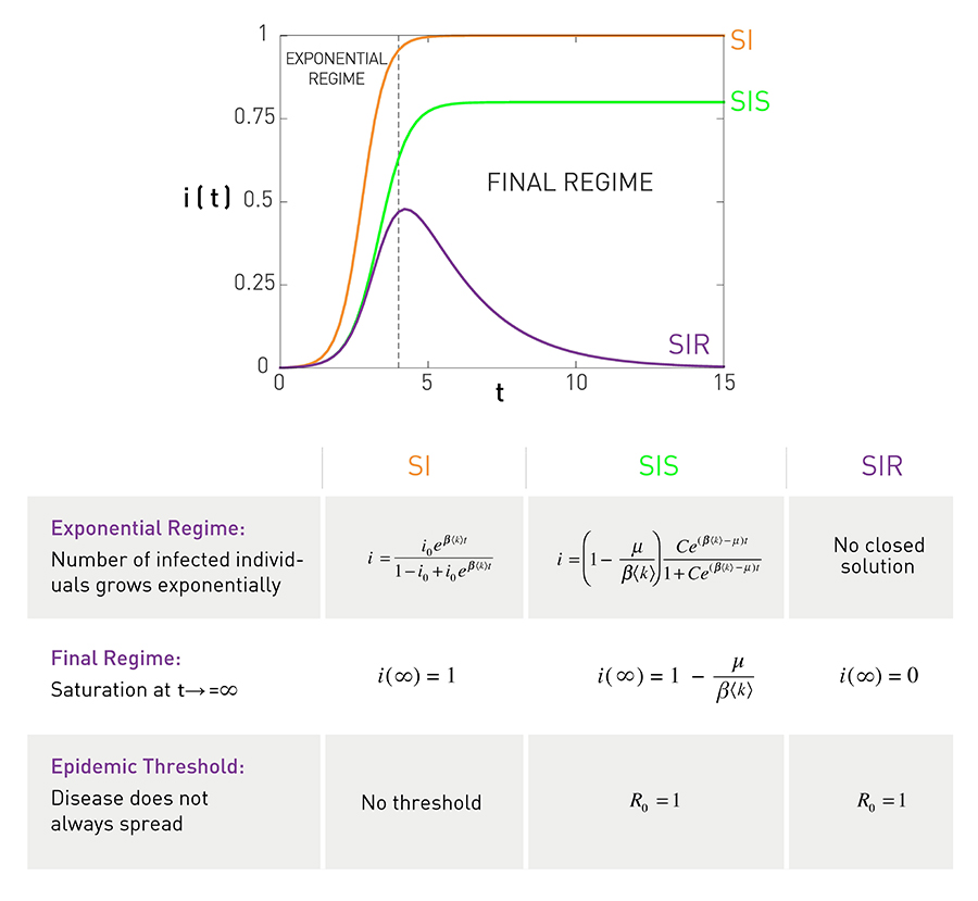
Comparing the SI, SIS and SIR Models
The plot shows growth of the fraction of infected individuals, i, in the SI, SIS and SIR models. Two different regimes stand out:
Exponential Regime
The models predict an exponential growth in the number of infected individuals during the early stages of the epidemic. For the same β the SI model predicts the fastest growth (smallest τ, see (10.5)). For the SIS and SIR models the growth is slowed by recovery, resulting in a larger τ, as predicted by (10.9). Note that for sufficiently high recovery rate μ the SIS and the SIR models predict a disease-free state, when the number of infected individuals decays exponentially with time.
Final Regime
The three models predict different long-term outcomes: In the SI model everyone becomes infected, i(∞)=1; in the SIS model a finite fraction of individuals are infected i(∞) < 1; in the SIR model all infected nodes recover, hence the number of infected individuals goes to zero i(∞)=0.
The table summarizes the main properties of each model.
Section 10.3
Network Epidemics
The ease of air travel, allowing millions to cross continents on a daily basis, has dramatically accelerated the speed with which pathogens travel around the world. While in medieval times a virus took years to sweep a continent (Image 10.8), today a new virus can reach several continents in a matter of days. There is an acute need, therefore, to understand and predict the precise patterns that pathogens follow as they spread around the globe.
Image 10.8
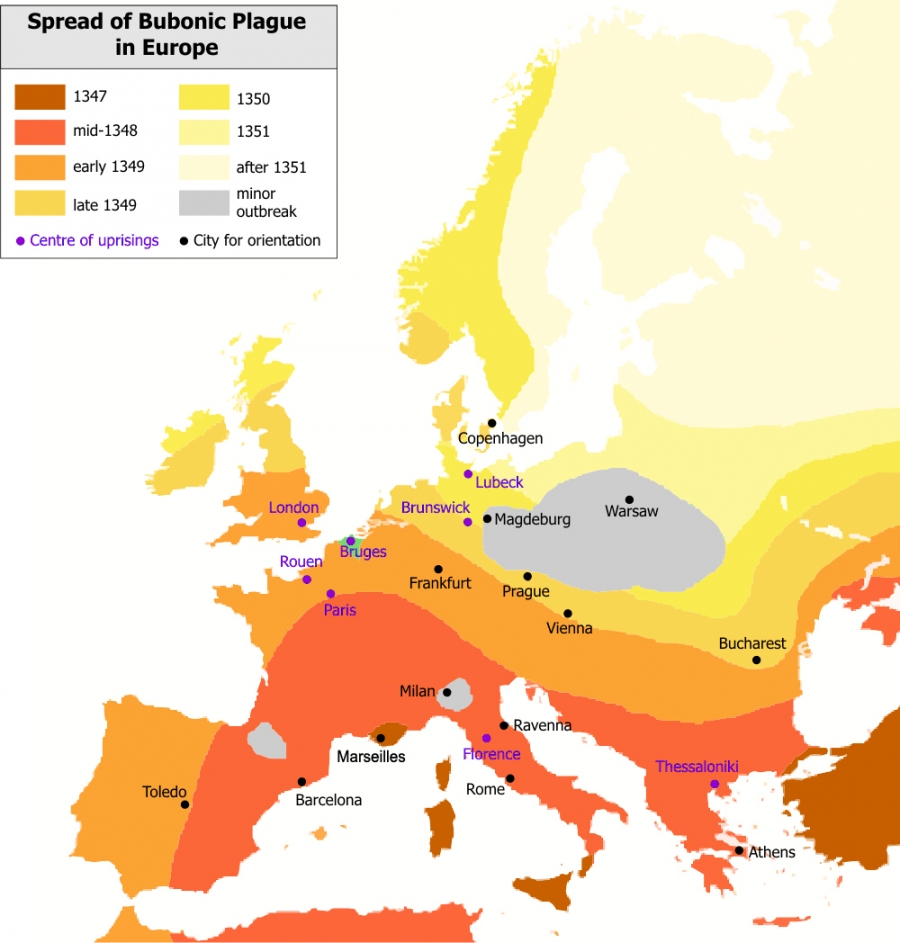
The Great Plague
The Black Death, one of the most devastating pandemics in human history, was an outbreak of bubonic plague caused by the bacterium Yersinia pestis. The figure shows the gradual advance of the disease throughout Europe, taking years to sweep the continent. It started in China and traveled along the Silk Road to reach Crimea around 1346. From there, probably carried by Oriental rat fleas on the black rats that were regular passengers on merchant ships, spread throughout the Mediterranean and Europe. Its slow spread reflected the slow travel speed of its era. The black death is estimated to have killed 30% to 60% of Europe's population [8]. The resulting devastation has caused a series of religious, social and economic upheavals, having a profound impact on the history of Europe.
After Roger Zenner, Wikipedia.
The epidemic models discussed in the previous section do not incorporate the structure of the contract network that facilitates the spread of a pathogen. Instead they assume that any individual can come into contact with any other individual (homogenous mixing hypothesis) and that all individuals have comparable number of contacts, 〈k〉. Both assumptions are false: Individual can transmit a pathogen only to those they come into contact with, hence pathogens spread on a complex contact network. Furthermore, these contact networks are often scale-free, hence 〈k〉 is not sufficient to characterize their topology.
The failure of the basic hypotheses prompted a fundamental revision of the epidemic modeling framework. This change began with the work of Romualdo Pastor-Satorras and Alessandro Vespignani, who in 2001 extended the basic epidemic models to incorporate in a self-consistent fashion the topological characteristics of the underlying contact network [9]. In this section we introduce the formalism developed by them, familiarizing ourselves with network epidemics.
Susceptible-Infected (SI) Model on a Network
If a pathogen spreads on a network, individuals with more links are more likely to be in contact with an infected individual, hence they are more likely to be infected. Therefore the mathematical formalism must consider the degree of each node as an implicit variable. This is achieved by the degree block approximation, that distinguishes nodes based on their degree and assumes that nodes with the same degree are statistically equivalent (Image 10.9). Therefore we denote with
the fraction of nodes with degree k that are infected among all Nk degree-k nodes in the network. The total fraction of infected nodes is the sum of all infected degree-k nodes
Given the different node degrees, we write the SI model for each degree k/ separately:
This equation has the same structure as (10.3): The infection rate is proportional to β and the fraction of degree-k nodes that are not yet infected, which is (1-ik). Yet, there are some key differences:
The average degree 〈k〉 in (10.3) is replaced with each node’s actual degree k.
The density function Θk represents the fraction of infected neighbors of a susceptible node k. In the homogenous mixing assumption Θk is simply the fraction of the infected nodes, i. In a network environment, however, the fraction of infected nodes in the vicinity of a node can depend on the node’s degree k and time t.
While (10.3) captures with a single equation the time dependent behavior of the whole system, (10.13) represents a system of kmax coupled equations, one equation for each degree present in the network.
Image 10.9
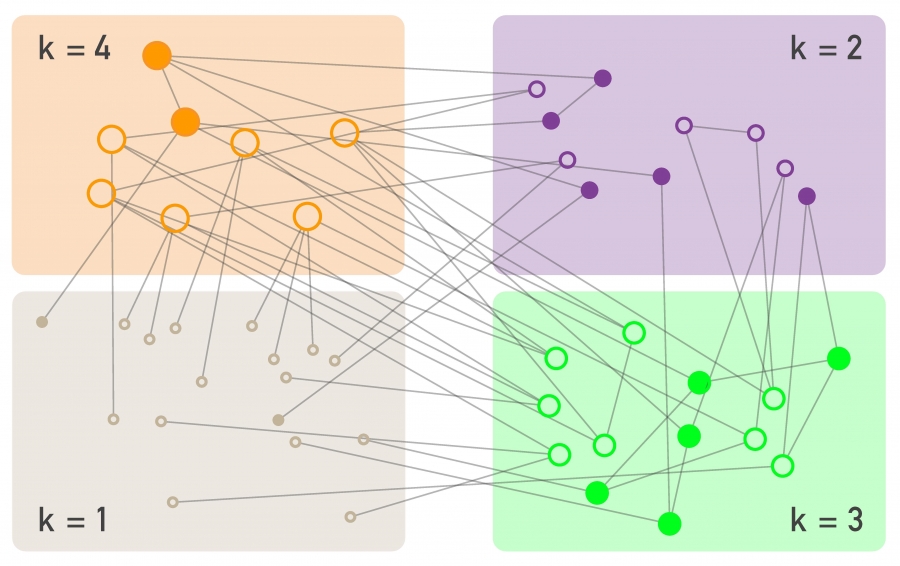
Degree Block Approximation
The epidemic models discussed in SECTION 10.2 grouped each node into compartments based on their state, placing them into susceptible, infected, or recovered compartments. To account for the role of the network topology, the degree block approximation adds an additional set of compartments, placing all nodes that have the same degree into the same block. In other words, we assume that nodes with the same degree behave similarly. This allows us to write a separate rate equation for each degree, as we did in (10.13). The degree block approximation does not eliminate the compartments based on the state of an individual: Independent of its degree an individual can be susceptible to the disease (empty circles) or infected (full circles).
We start by exploring the early time behavior of ik, a choice driven by both theoretical interest and practical considerations. Indeed, developing vaccines, cures, and other medical interventions for a new pathogen can take months to years. If we lack a cure, the only way to alter the course of an epidemic is to do so early, using quarantine, travel restrictions and transmission-slowing measures to halt its spread. To make the right decision about the nature, the timing and the magnitude of each intervention, we need an accurate estimate of the number of individuals infected in the early stages of the epidemic.
At the beginning of the epidemic ik is small and the higher order term in (10.13) βikkΘk can be neglected. Hence we can approximate (10.13) with
As we show in ADVANCED TOPICS 10.B, for a network lacking degree correlations the Θk function is independent of k, so using (10.40), (10.14) becomes
where τSI is the characteristic time for the spread of the pathogen
Integrating (10.15) we obtain the fraction of infected nodes with degree k
Equation (10.17) makes several important predictions:
The higher the degree of a node, the more likely that it becomes infected. Indeed, for any time t we can write (10.17) as ik=g(t)+kf(t), indicating that the group of nodes with higher degree has a higher fraction of infected nodes (Figure 10.10).
According to (10.12) the total fraction of infected nodes grows with time as
According to (10.16) the characteristic time τ depends not only on 〈k〉, but also on the network’s degree distribution through 〈k2〉. To fully understand the significance of the prediction (10.16), let us derive τSI for different networks:
Random Network
For a random network 〈k2〉=〈k〉(〈k〉+1), obtaining
recovering the result (10.5) for homogenous networks.
Scale-free Network with γ≥3
If the contract network on which the disease spreads is scale-free with degree exponent γ ≥3, both 〈k〉 and 〈k2〉 are finite. Consequently τSI is also finite and the spreading dynamics is similar to the behavior predicted for a random network but with an altered τSI.
Scale-free Networks with γ≤3
For γ < 3 in the N→∞ limit 〈k2〉→∞ hence (10.16) predicts τSI→0. In other words, the spread of a pathogen on a scale-free network is instantaneous. This is perhaps the most unexpected prediction of network epidemics.
The vanishing characteristic time reflects the important role hubs play in epidemic phenomena. Indeed, as illustrated in Image 10.10, in a scale-free network the hubs are the first to be infected, as through the many links they have, they are very likely to be in contact with an infected node. Once a hub becomes infected, it “broadcasts” the disease to the rest of the network, turning into a super-spreader.
Inhomogenous Networks
A network does not need to be strictly scale-free for the impact of the degree heterogeneity to be detectable. Indeed, (10.16) predicts that as long as 〈k2〉 > 〈k〉(〈k〉+1), τSI is reduced. Hence heterogenous network enhance the speed of any pathogen.
Image 10.10
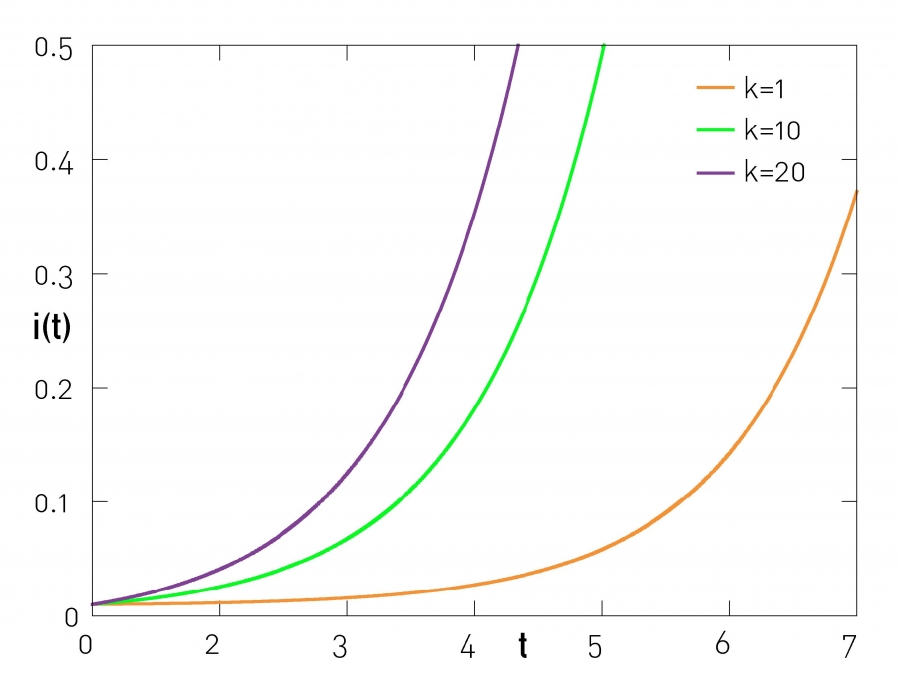
Fraction of Infected Nodes in the SI Model
Equation (10.17) predicts that the a pathogen spreads with different speed on nodes with different degrees. To be specific, we can write ik=g(t)+kf(t), indicating that at any time the fraction of high degree nodes that are infected is higher than the fraction of low degree nodes. The figure shows the fraction of infected nodes with degrees k=1, 10 and 100 in an Erdős-Rényi network with average degree 〈k〉=2. It shows that at t=3 less than 3% of the k=1 nodes are infected, in contrast with close to 20% of the k=10 nodes and close to 30% of the k=20 nodes. Consequently, at any time virtually all hubs are infected, but small-degree nodes tend to be disease free. Hence the disease is maintained in the hubs, which in turn broadcast the disease to the rest of the network.
In the SI model with time the pathogen reaches all individuals. Consequently the degree heterogeneity affects only the characteric time, which in turn determines the speed with which the pathogen sweeps through the population. To understand the full impact of the network topology, we need to explore the behavior of the SIS model on a network.
SIS Model and the Vanishing Epidemic Threshold
The continuum equation describing the dynamics of the SIS model on a network is a straightforward extension of the SI model discussed in SECTION 10.2,
The difference between (10.13) and (10.20) is the presence of the recovery term -µik. This changes the characteristic time of the epidemic to (ADVANCED TOPICS 10.B)
For sufficiently large µ the characteristic time is negative, hence ik decays exponentially. The condition for the decay depends not only on the recovery rate and 〈k〉, but also on the network heterogenity, through 〈k2〉. To predict when a pathogen persists in the population we define the spreading rate
which depends only on the biological characteristics of the pathogen, namely the transmission probability β and the recovery rate μ. The higher is λ, the more likely that the disease will spread. Yet, the number of infected individuals does not increase gradually with λ. Rather, the pathogen can spread only if its spreading rate exceeds an epidemic threshold λc. Next we calculate λc for random and scale-free networks.
Random Network
If a pathogen spreads on a random network, we can use 〈k2〉=〈k〉 (〈k+1〉) in (10.21), obtaining that the pathogen persists in the population if
Using (10.22) we obtain
obtaining the epidemic threshold of a random network as
As 〈k〉 is always finite, a random network always has a nonzero epidemic threshold (Image 10.11), with key consequences:
If the spreading rate λ exceeds the epidemic threshold λc, the pathogen will spread until it reaches an endemic state, where a finite fraction i(λ) of the population is infected at any time.
If λ < λc, the pathogen dies out, i.e. i(λ)=0.
Hence the epidemic threshold allows us to decide if a pathogen can or cannot persist in a population. This transition from the absence to the presence of an epidemic outbreak by increasing the spreading rate λ is at the basis of most campaigns to stop a pathogen (SECTION 10.6).
Image 10.11
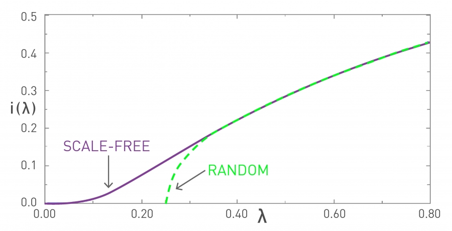
Epidemic Threshold
The fraction of infected individuals i(λ)=i(t→∞) in the endemic state of the SIS model. The curves are for a random (green) and for a scale-free contact network (purple). The random network has a finite epidemic threshold λc, implying that a pathogen with a small spreading rate (λ < λc) must die out, i.e. i(λc)=0. If, however, the spreading rate of the pathogen exceeds λc, the pathogen becomes endemic and a finite fraction of the population is infected at any time. For a scale-free network we have λc=0, hence even viruses with a very small spreading rate λ can persist in the population.
Scale-free Network
For a network with an arbitrary degree distribution we set τSIS > 0 in (10.21), obtaining the epidemic threshold as
As for a scale-free network 〈k2〉 diverges in the N→∞ limit, for large networks the epidemic threshold is expected to vanish (Image 10.11 and 10.12). This means that even viruses that are hard to pass from individual to individual can spread successfully, representing the second fundamental prediction of network epidemics.
Image 10.12
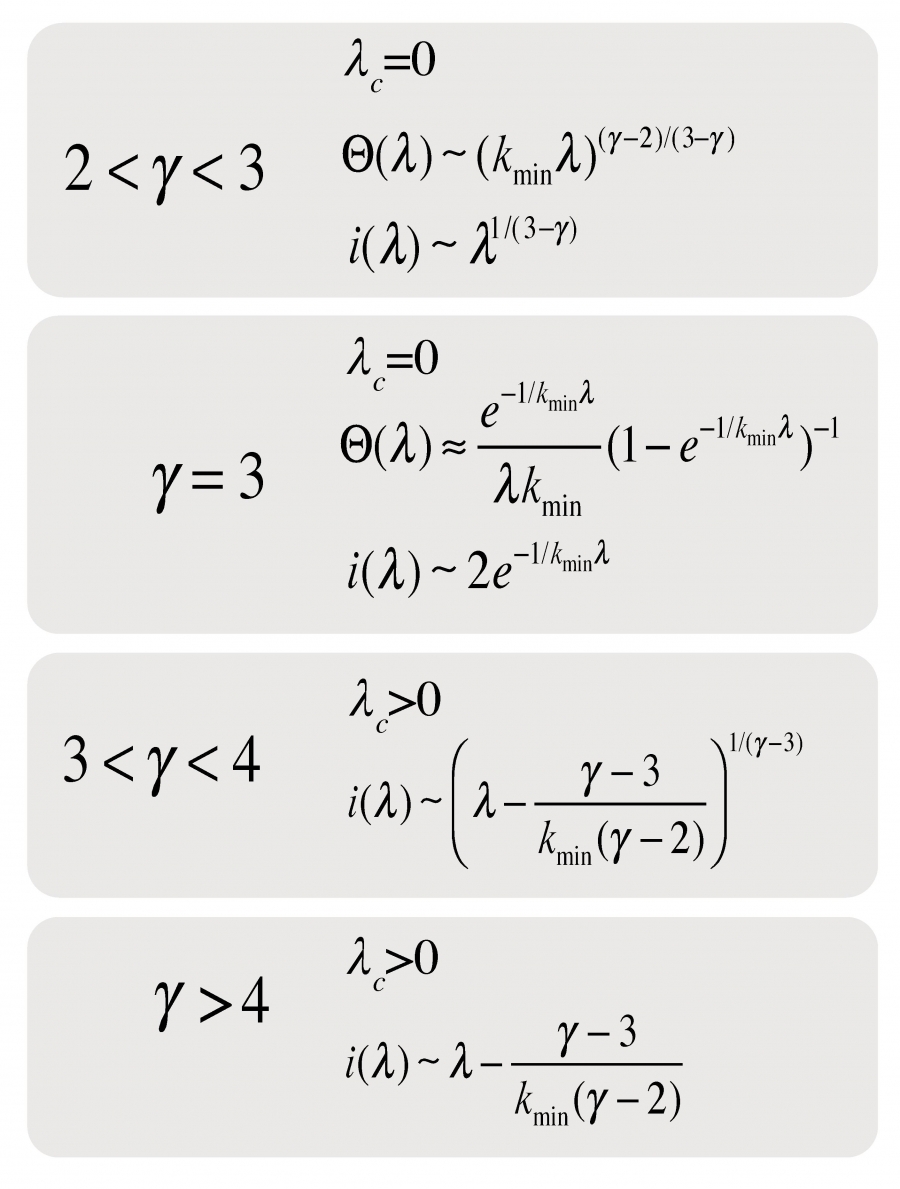
The Asymptotic Behavior of the SIS Model
The fraction of individuals infected in the endemic state, i(λ)=i(t→∞), depends on the structure of the underlying network and the disease parameters β and μ. The figure summarizes the key properties of the epidemic threshold λc, the density function Θ(λ) and i(λ) for a scale-free network with degree exponent γ. The results indicate that only for γ >4 does the epidemics on a scale-free network converge to the results of the traditional epidemic models. After [10].
The vanishing epidemic threshold is a direct consequence of the hubs. Indeed, a pathogen that fails to infect other nodes before the infected individual recovers, will slowly disappear from the population (ADVANCED TOPICS 10.A). In a random network all nodes have comparable degree, k≈〈k〉, hence if the spreading rate is under the epidemic threshold, the pathogen has no avenues to spread. In a scale-free network, however, even if a pathogen is only weakly infectious, if it infects a hub, the hub can pass it on to a large number of other nodes, allowing it to persist in the population.
In summary, the results of this section show that accounting for the network topology greatly alters the predictive power of the epidemic models. We derived two fundamental results:
In a large scale-free network τ=0, which means that a virus can instantaneously reach most nodes.
In a large scale-free network λc=0, which means that even viruses with small spreading rate can persist in the population.
Both results are the consequence of hubs’ ability to broadcast a pathogen to a large number of other nodes.
Model
Continuum Equation
τ
λc
SI
0
SIS
SIR
Table 10.3
Epidemic Models on Networks
The table shows the rate equation for the three basic epidemic models (SI, SIS, SIR) on a network with arbitrary 〈k〉 and 〈k2〉, together with the corresponding characteristic τ and the epidemic threshold λc. For the SI model λc =0, as in the absence of recovery (µ=0) a pathogen spreads until it reaches all susceptible individuals. The listed τ and λc are derived in ADVANCED TOPICS 10.B.
Note that these results are not limited to scale-free networks. Rather (10.16) and (10.26) predict that both τ and λc depend on 〈k2〉, hence the effects discussed above will impact any network with high degree heterogeneity. In other words, if 〈k2〉 is larger than the random expectation 〈k〉(〈k+1〉), we will observe an enhanced spreading process, resulting in a smaller τ and λc than predicted by the traditional epidemic models. As this implies a faster spread of the pathogen than predicted by the traditional epidemic models, efforts to control an epidemic cannot ignore this difference.
The results of this section were based on the degree-block approximation, which treats the detailed time-dependent infection process in a mean-field fashion. Note, however, that this approximation, while simplifies the presentation, is not necessary. The underlying stochastic problem can be treated in its full mathematical complexity [11-14]. Such calculations show that due to the fact that the hubs can be re-infected in the SIS model, the epidemic threshold vanishes even for γ >3, in contrast with the finite threshold predicted by the mean-field approach (Image 10.12). Hence hubs play an even more important role than our earlier calculations indicate.
Section 10.4
Contact Networks
Network epidemics predicts that the speed with which a pathogen spreads depends on the degree distribution of the relevant contact network. Indeed, we found that 〈k2〉 affects both the characteristic time τ and the epidemic threshold λc. None of these findings are consequential if the network on which a pathogen spreads is random - in that case the predictions of network epidemics are indistinguishable from the predictions of the traditional epidemic models encountered in SECTION 10.2. In this section we inspect the structure of several contact networks encountered in epidemic phenomena, offering direct empirical evidence of the significance of the underlying degree heterogeneities.
Sexually Transmitted Diseases
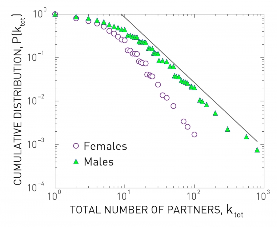
The HIV virus, the pathogen responsible for AIDS, spreads mainly through sexual intercourse. Consequently, the relevant contact network captures who had sexual relationship with whom. The structure of this sex web was first revealed by a study surveying the sexual habits of the Swedish population [15]. Through interviews and questionnaires, researchers collected information from 4,781 randomly chosen Swedes of ages 18 to 74. The participants were not asked to reveal the identity of their sexual partners, but only to estimate the number of sexual partners they had during their lifetime. Hence the researchers could reconstruct the degree distribution of the sexual network [16], finding that it is well approximated with a power law (Image 10.13). This was the first empirical evidence of the relevance of scale-free networks to the spread of pathogens. The finding was confirmed by data collected in Britain, US and Africa [17].
The scale-free nature of the sexual network indicates that most individuals have relatively few sexual partners. A few individuals, however, had hundreds of sexual partners during their lifetime. Consequently the sexual network has a high 〈k2〉, which lowers both τ and λc.
Image 10.13
The Sex Web
Cumulative distribution of the total number of sexual partners k since sexual initiation for individuals interviewed in the 1996 study on sexual patterns in Sweden [15]. For women a power law fit to the tail indicates γ=3.1±0.3 for k > 20; for men γ=2.6±0.3 in the range 20 < k < 400. Note that for men the average number of partners is higher than for women. This difference may be rooted social bias, prompting males to exaggerate and females to suppress the number of sexual partners they report. After [16].
Airborne Diseases
For airborne diseases, like influenza, SARS or H1N1, the contact network captures the set of individuals a person comes into physical proximity. The structure of this contact network is explored at two levels. First, the global travel network allows us to predict the worldwide spread of a pathogen, representing the input of several large-scale epidemic prediction tools (SECTION 10.7). Second, digital badges probe the local properties of the contact network, i.e. the number of individuals a person directly interacts with.
Global Travel Network
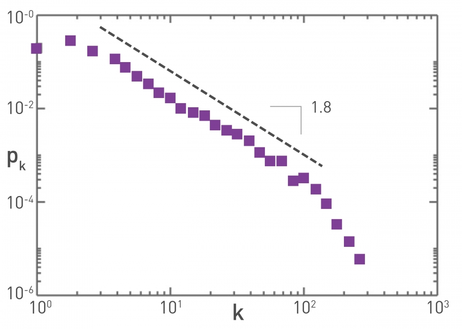
To predict the spread of pathogens, we must know how far infected individuals travel. Our understanding of individual travel patterns exploded with the use of mobile phones, that offer direct information about individual mobility [21-24]. In the context of epidemic phenomena, the most studied mobility data comes from air travel, the mode of transportation that determines the speed with which a pathogen moves around the globe. Consequently the air transportation network, that connects airports with direct flights, plays a key role in modeling and predicting the spread of pathogens [25-27]. As Image 10.15 shows, this network is scale-free with degree exponent γ=1.8. This low value is possible because there are multiple flights between two airports, hence the network is not simple. A similar power law distribution is detected for the link weights, indicating that the number of passengers traveling between two airports is typically low, but between some airports the traffic can be extraordinary. As we discuss in SECTION 10.5, these heterogeneities play a key role in the spread of specific pathogens.
Image 10.15
Air Transportation Network
The degree distribution of the air transportation network is well approximated by a power-law with γ =1.8 ±0.2. The map was built using the International Air Transport Association database that contains the world list of airport and the direct flights between them in 2002. The resulting network is a weighted graph containing the N=3,100 largest airports as nodes that are connected by L=17,182 direct flights as links, together accounting for 99% of the worldwide traffic. After [25].
Local Contact Patterns
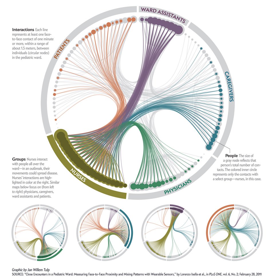
Many airborne diseases spread thanks to face-to-face interactions [28-31]. These interaction patterns can be monitored using Radio-Frequency Identification Devices (RFID) [29,31], mobile-phone based sociometric badges [32,33], and other wireless technologies [34].
Video 10.1 Detecting Networks via RFIDs
A video introducing the RFID technology and their use in mapping social interactions.
RFID are digital badges that detect the proximity of other individuals that wear a badge (Video 10.1). They have been deployed in various environment, capturing for example the interactions between more than 14, 000 visitors of a Science Gallery over a three month period or between 100 participants of a three-day conference [29]. An RFID-mapped network shown in Image 10.16 captures the interactions between high school students and their teachers during a two-day period. Several findings stand out:
RFID tags detect interactions only with individuals that wear the same badge and face each other, limiting the number of detected contacts. Consequently the contact networks mapped out in these studies typically have an exponential degree distribution.
The duration of each face-to-face interaction follows a power law distribution over several orders of magnitude. Therefore most contacts are brief, but there are a few lasting interactions, documenting bursty temporal pattern [35] with key consequences for the spread of pathogens (SECTION 10.5).
The link weights, which capture the cumulative time two individuals have spent together, also follow a power law distribution. Therefore individuals spend most of their time with only a few others, again with important implications on spreading patterns (SECTION 10.5).
For most airborne pathogens spatial proximity is sufficient for transmission. For example, standing next to an infected individual in the elevator may be sufficient to transmit SARS or H1N1, an interaction not recorded by a RFID tag.
In summary, RFID tags provide remarkably detailed temporal and spatial information about local contacts. To be useful these studies must be scaled up, using for example mobile phone based technologies [36].
Image 10.16
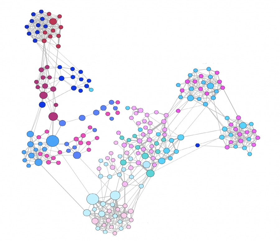
AFace-to-face Interactions
A face-to-face contact network mapped out using RFA tags, capturing interactions between 232 students and 10 teachers across 10 classes in a school [31]. The structure of the maps obtained by RFID tags depend on the context in which they are collected. For example the school network shown here reveals the presence of clear communities. In contrast, a study capturing the interactions between individuals that visited a museum reveal an almost linear network [29]. Finally, a network of attendees of a small conference is rather dense, as most participants interact with most others [29]. After [31].
Location Networks
For many airborne pathogens the relevant contact network is the socalled location network, whose nodes are the locations that are connected by individuals that move regularly between them. Measurements combined with agent-based simulations indicate that the location network is fat tailed [37]: malls, airports, schools or supermarkets act as hubs, being linked to an exceptionally large number of smaller locations, like homes and offices. Therefore, once the pathogen infects a hub, the disease can rapidly reach many other locations.
Digital Viruses
The study of digital viruses, that infect computers and smart phones, represents an increasingly important application of epidemic phenomena. As we discuss next, the relevent contact networks are determined by the spreading mode of the respective digital pathogen.
Computer Viruses
Computer viruses display just as much diversity as biological viruses: depending on the nature of the virus and its spreading mechanism, the relevant contact network can differ dramatically. Many computer viruses spread as email attachments. Once a user opens the attachment, the virus infects the user’s computer and mails a copy of itself to the email addresses found in the computer. Hence the pertinent contact network is the email network, which, as we discussed in Table 4.1, is scale-free [58]. Other computer viruses exploit various communication protocols, spreading on networks that reflect the Internet's pattern of interconnectedness, which is again scale-free (Table 4.1). Finally, some malware scan IP addresses, spreading on fully connected networks.
Mobile Phone Viruses
Mobile phone viruses spread via MMS and Bluetooth (Image 10.2). An MMS virus sends a copy of itself to all phone numbers found in the phone's contact list. Therefore MMS viruses exploit the social network behind mobile communications. As shown in Table 4.1, the mobile call network is scale-free with a high degree exponent. Mobile viruses can also spread via Bluetooth, passing a copy of themselves to all susceptible phones with a BT connection in their physical proximity. As discussed above, this co-location network is also highly heterogenous [4].
In summary, in the past decade technological advances allowed us to map out the structure of several networks that support the spread of biological or digital viruses, from sexual to proximity-based contact networks (see also Online Resource 10.2). Many of these, like the email network, the internet, or sexual networks, are scale-free. For others, like co-location networks, the degree distribution may not be fitted with a simple power law, yet show significant degree heterogeneity with high 〈k2〉. This means that the analytical results obtained in the previous section are of direct relevance to pathogens spreading on most networks. Consequently the underlying heterogenous contact networks allow even weakly virulent viruses to easily spread in the population.
Online Resource 10.2 Hospital Outbreaks
Bacteria resistant to current antibiotics pose an important threat to global health. Such bacteria are particularly prevalent in hospitals and health care facilities. The Interactive Feature by Scientific American describes the tracking of bacterical outbreaks in hospitals.
Section 10.5
Beyond the Degree Distribution
So far we have kept our models simple: We assumed that pathogens spread on an unweighted network uniquely defined by its degree distribution. Yet, real networks have a number of characteristics that are not captured by pk alone, like degree correlations or community structure. Furthermore, the links are typically weighted and the interactions have a finite temporal duration. In this section we explore the impact of these properties on the spread of a pathogen.
Temporal Networks
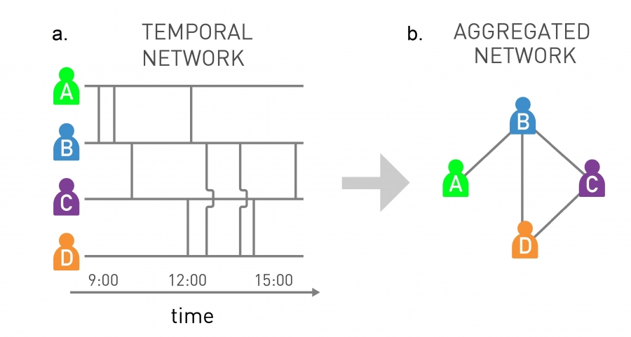
Most interactions that we perceive as social links are brief and infrequent. As a pathogen can be only transmitted when there is an actual contact, an accurate modeling framework must also consider the timing and the duration of each interaction. Ignoring the timing of the interactions can lead to misleading conclusions [39-41]. For example, the static network of Image 10.17b was obtained by aggregating the individual interactions shown in Image 10.17a. On the aggregated network the infection has the same chance of spreading from D to A as from A to D. Yet, by inspecting the timing of each interaction, we realize that while an infection starting from A can infect D, an infection that starts at D cannot reach A. Therefore, to accurately predict an epidemic process we must consider the fact that pathogens spread on temporal networks, a topic of increasing interest in network science [40-43]. By ignoring the temporality of these contact patterns, we typically overestimate the speed and the extent of an outbreak [42,43].
Image 10.17
Temporal Networks
Most interactions in a network are not continuous, but have a finite duration. We must therefore view the underlying networks as temporal networks, an increasingly active research topic in network science.
Temporal Network
The timeline of the interactions between four individuals. Each vertical line marks the moment when two individuals come into contact with each other. If A is the first to be infected, the pathogen can spread from A to B and then to C, eventually reaching D. If, however, D is the first to be infected, the disease can reach C and B, but not A. This is because there is a temporal path from A to D.
Aggregated Network
The network obtained by merging the temporal interactions shown in (a). If we only have access to this aggregated representation, the pathogen can reach all individuals, independent of its starting point. After [40].
Bursty Contact Patterns
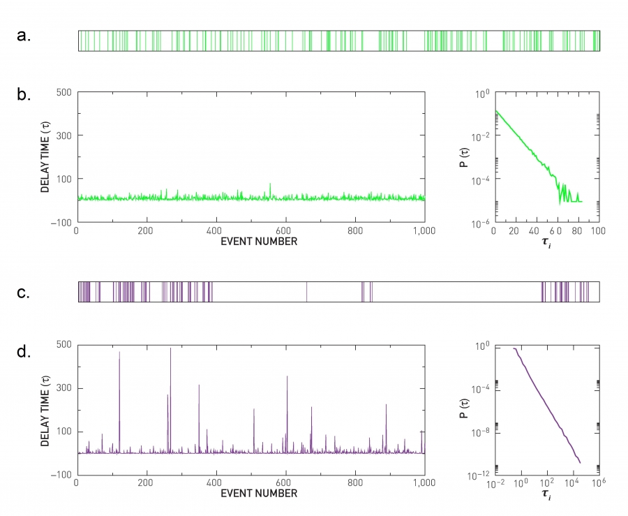
The theoretical approaches discussed in the SECTIONS 10.2 and 10.3 assume that the timing of the interactions between two connected nodes is random. This means that the interevent times between consecutive contacts follow an exponential distribution, resulting in a random but uniform sequence of events (Image 10.18a-c). The measurements indicate otherwise: The interevent times in most social systems follow a power law distribution [35,44] (Image 10.18d-f). This means that the sequence of contacts between two individuals is characterized by periods of frequent interactions, when multiple contacts follow each other within a relatively short time frame. Yet, the power law also implies that occasionally there are a very long time gaps between two contacts. Therefore the contact pattern have an uneven, “bursty” character in time (Image 10.18d,e).
Image 10.18
Bursty Interactions
If the pattern of activity of an individual is random, the interevent times follow a Poisson process, which assumes that in any moment an event takes place with the same probability q. The horizontal axis denotes time and each vertical line corresponds to an event whose timing is chosen at random. The observed inter-event times are comparable to each other and very long delays are rare.
The absence of long delays is visible if we show the inter-event times τi for 1,000 consecutive random events. The height of each vertical line corresponds to the gaps seen in (a).
The probability of finding exactly n events within a fixed time interval follows the Poisson distribution P(n,q)=e–qt(qt)n/n!, predicting that the inter-event time distribution follows P(τi)~e–qτi, shown on a log-linear plot.
The succession of events for a temporal pattern whose interevent times follow a power-law distribution. While most events follow each other closely, forming bursts of activity, there are a few exceptionally long interevent times, corresponding to long gaps in the contact pattern. The time sequence is not as uniform as in (a), but has a bursty character.
The waiting time τi of 1,000 consecutive events, where the mean event time is chosen to coincide with the mean event time of the Poisson process shown in (b). The large spikes correspond to exceptionally long delays.
The delay time distribution P(τi)~τi–2 for the bursty process shown in (d) and (e). After [35].
Bursty interactions are observed in a number of contact processes of relevance for epidemic phenomena, from email communications to call patterns and sexual contacts. Once present, burstiness alters the dynamics of the spreading process [43]. To be specific, power law interevent times increase the characteristic time τ, consequently the number of infected individuals decays slower than predicted by a random contact pattern. For example, if the time between consecutive emails would follow a Poisson distribution, an email virus would decay following i(t)~exp(–t/τ) with a decay time of τ≈1 day. In the real data, however, the decay time is τ≈21 days, a much slower process, correctly predicted by the theory if we use power law interevent times [43].
Degree Correlations
As discussed in CHAPTER 7, many social networks are assortative, implying that high degree nodes tend to connect to other high degree nodes. Do these degree correlations affect the spread of a pathogen? The calculations indicate that degree correlations leave key aspects of network epidemics in place, but they alter the speed with which a pathogen spreads in a network:
Degree correlations alter the epidemic threshold λc: assortative correlations decrease λc and dissasortative correlations increase it [45,46].
Despite the changes in λc, for the SIS model the epidemic threshold vanishes for a scale-free network with diverging second moment, whether the network is assortative, neutral or disassortative [47]. Hence the fundamental results of SECTION 10.3 are not affected by degree correlations.
Given that hubs are the first to be infected in a network, assortativity accelerates the spread of a pathogen. In contrast disassortativity slows the spreading process.
Finally, in the SIR model assortative correlations were found to lower the prevalence but increase the average lifetime of an epidemic outbreak [48].
Link Weights and Communities
Throughout this chapter we assumed that all tie strengths are equal, focusing our attention on pathogens spreading on an unweighted network. In reality tie strengths vary considerably, a heterogeneity that plays an important role in spreading phenomena. Indeed, the more time an individual spends with an infected individual, the more likely that she too becomes infected.
In the same vein, previously we ignored the community structure of the network on which the pathogen spreads. Yet, the existence communities (CHAPTER 9) leads to repeated interactions between the nodes within the same community, altering the spreading dynamics.
The mobile phone network allows us to explore the role of tie strengths and communities on spreading phenomena [49]. Let us assume that at t=0 we provide a randomly selected individual with some key information. At each time step this “infected” individual i passes the information to her contact j with probability pij~βwij, where β is the spreading probability and wij is the strength of the ties captured by the number of minutes i and j have spent with each other on the phone. Indeed, the more time two individuals talk, the higher is the chance that they will pass on the information. To understand the role of the link weights in the spreading process, we also consider the situation when the spreading takes place on a control network, that has the same wiring diagram but all tie strengths are set equal to w=〈wij〉.
As Image 10.19a illustrates, information travels significantly faster on the control network. The reduced speed observed in the real system indicates that the information is trapped within communities. Indeed, as we discussed in CHAPTER 9, strong ties tend to be within communities while weak ties are between them [50]. Therefore, once the information reaches a member of a community, it can rapidly reach all other members of the same community, given the strong ties between them. Yet, as the ties between the communities are weak, the information has difficulty escaping the community. Consequently the rapid invasion of the community is followed by long intervals during which the infection is trapped within a community. When all link weights are equal (control), the bridges between communities are strengthened, and the trapping vanishes.
Image 10.19
Information Diffusion in Mobile Phone Networks
The spread of information on a weighted mobile call graph, where the probability that a node passes information to one of its neighbors is proportional to the strength of the tie between them. The tie strength is the number of minutes two individuals talk on the phone.
The fraction of infected nodes in function of time. The blue circles capture the spread on the network with the real tie strengths; the green symbols represent the control case, when all tie strengths are equal.
Spreading in a small network neighborhood, following the real link weights. The information is released from the red node, the arrow weight indicating the tie strength. The simulation was repeated 1,000 times; the size of the arrowheads is proportional to the number of times the information was passed along the corresponding direction, and the color indicates the total number of transmissions along that link. The background contours highlight the difference in the direction the information follows in the real and the control simulations.
Same in (b), but we assume that each link has the same weight w=〈wij〉(control). After [49].
The difference between the real and the control spreading process is illustrated by Image 10.20b,c, that shows the spreading pattern in a small neighborhood of the mobile call network. In the control simulation the information tends to follow the shortest path. When the link weights are taken into account, information flows along a longer backbone with strong ties. For example, the information rarely reaches the lower half of the network in Image 10.20b, a region always reached in the control simulation shown in (c).
Image 10.20
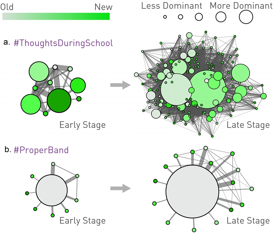
Simple vs. Complex Contagion
The community structure of the Twitter follower network. Each circle corresponds to a community and its size is proportional to the number of tweets produced by the respective community. The color of a community represents the time when the studied hashtag (meme) is first used in the community. Lighter colors denote the first communities to use a hashtag, darker colors denote the last community to adapt it.
Simple Contagion
The evolution of the viral meme captured by the #ThoughtsDuringSchool hashtag from its early stage (30 tweets, left) to the late stage (200 tweets, right). The meme jumps easily between communities, infecting many of them, following a contagion pattern encountered in the case of biological pathogens.
Complex Contagion
The evolution of a non-viral meme caputed by the #ProperBand hashtag from the early stage (left) to the final stage (65 tweets, right). The tweet is trapped in a few of communities, having difficulty to escape them. This is a signature of reinforcement, an indication that the meme follows complex contagion. After [54].
Complex Contagion
Communities have multiple consequences for spreading, from inducing global cascades [51,52] to altering the activity of individuals [53].
The diffusion of memes, representing ideas or behavior that spread from individual to individual, further highlights the important role of communities [54]. Meme diffusion has attracted considerable attention from marketing [5, 55] to network science [56,57], communications [58], and social media [59-61]. Pathogens and memes can follow different spreading patterns, prompting us to systematically distinguish simple from complex contagion [54,62,63].
Simple contagion is the process we explored so far: It is sufficient to come into contact with an infected individual to be infected. The spread of memes, products and behavior is often described by complex contagion, capturing the fact that most individuals do not adopt a new meme, product or behavioral pattern at the first contact. Rather, adoption requires reinforcement [64], i.e. repeated contact with several individuals who have already adopted. For example, the higher is the fraction of a person’s friends that have a mobile phone, the more likely that she also buys one.
In simple contagion communities trap an information or a pathogen, slowing the spreading (Image 10.19a). The effect is reversed in complex contagion: Because communities have redundant ties, they offer social reinforcement, exposing an individual to multiple examples of adoption. Hence communities can incubate a meme, a product or a behavioral pattern, enhancing its adoption.
The difference between simple and complex contagion is well captured by Twitter data. Tweets, or short messages, are often labeled with hashtags, which are keywords acting as memes. Twitter users can follow other users, receiving their messages; they can forward tweets to their own followers (retweet), or mention others in tweets. The measurements indicate that most hashtags are trapped in specific communities, a signature of complex contagion [54]. A high concentration of a meme within a certain community is evidence of reinforcement. In contrast, viral memes spread across communities, following a pattern similar to that encountered in biological pathogens. In general the more communities a meme reaches, the more viral it is (Image 10.20).
In summary, several network characteristics can affect the spread of a pathogen in a network, from degree correlations to link weights and the bursty nature of the contact pattern. As we discussed in this section, some network characteristics slow a pathogen, others aid their spread. These effects must therefore be accounted for if we wish to predict the spread of a real pathogen. While these patterns are of obvious relevance for infectious diseases, they also influence the spread of such non-infectious diseases as obesity (BOX 10.2).
Section 10.6
Immunization
Immunization strategies specify how vaccines, treatments or drugs are distributed in the population. Ideally, should a treatment or vaccine exist, it should be given to every infected individual or those at risk of contracting the pathogen. Yet, often cost considerations, the difficulty of reaching all individuals at risk, and real or perceived side effects of the treatment prohibit full coverage. Given these constraints, immunization strategies aim to minimize the threat of a pandemic by most effectively distributing the available vaccines or treatments.
Immunization strategies are guided by an important prediction of the traditional epidemic models: If a pathogen’s spreading rate λ is reduced under its critical threshold λc, the virus naturally dies out (Image 10.11). Yet, the epidemic threshold vanishes in scale-free networks, questioning the effectiveness of this strategy. Indeed, if the epidemic threshold vanishes, immunization strategies can not move λ under λc. In this section we discuss how to use our understanding of the network topology to design effective network-based immunization strategies that counter the impact of the vanishing epidemic threshold.
Random Immunization
The main purpose of immunization is to protect the immunized individual from an infection. Equally important, however, is its secondary role: Immunization reduces the speed with which the pathogen spreads in a population. To illustrate this effect consider the situation when a randomly selected g fraction of individuals are immunized in a population [8].
Let us assue that the pathogen follows the SIS model (10.3). The immunized nodes are invisible to the pathogen, and only the remaining (1–g) fraction of the nodes can contact and spread the disease. Consequently, the effective degree of each susceptible node changes from 〈k〉 to 〈k〉 (1–g), which decreases the spreading rate of the pathogen from λ= β/µ to λ'=λ(1–g). Next we explore the consequences of this reduction in both random and scale-free contact networks.
Random Networks
If the pathogen spreads on a random network, for a sufficiently high g the spreading rate λ' could fall below the epidemic threshold (10.25). The immunization rate gc necessary to achieve this is calculated by setting
obtaining
Consequently, if vaccination increases the fraction of immunized individuals above gc, it pushes the spreading rate under the epidemic threshold λc. In this case τ becomes negative and the pathogen dies out naturally. This explains why health official encourage a high fraction of the population take the influenza vaccine: The vaccine protects not only the individual, but also the rest of the population by decreasing the pathogen’s spreading rate. Similarly, a condom not only protects the individual who uses it from contacting the HIV virus, but also decrease the rate at which AIDS spreads in the sexual network. Hence for random networks a sufficiently high immunization rate can eliminate the pathogen from the population.
Heterogenous Networks
If the pathogen spreads on a network with high 〈k2〉, and random immunization changes λ to λ(1–g), we can use (10.26) to determine the critical immunization gc
obtaining
For a random network (10.29) reduces to (10.27). For a scale-free network with γ < 3 we have 〈k2〉→∞, hence (10.29) predicts gc →1. In other words if the contact network has a high 〈k2〉, we need to immunize virtually all nodes to stop the epidemic. This prediction is consistent with the finding that for many diseases we must immunize 80%-100% of the population to eradicate the pathogen. For example, measles requires 95% of the population to be immunized [8]; for digital viruses the strategies relying on random immunization call for close to 100% of the computers to install the appropriate antivirus software [67].
To illustrate the role degree heterogeneity plays in immunization let us consider a digital virus spreading on the email network. If we make the email network random and undirected, we have 〈k〉=3.26. Using λ=1 in (10.27) we obtain gc=0.76. In other words, to eradicate the virus we need to convince 76% of computer users to update their antivirus software. Yet, the email network is scalefree with 〈k2〉=1,271 (undirected version), hence (10.27) does not apply. In this case (10.29) predicts gc=0.997 for λ=1, meaning that more that 99.7% of the users must install the software to halt the email virus. It is virtually impossible to achieve this level of compliance - many users simply ignore all warnings. This is the reason why email viruses linger for years and disappear only after the operating systems that supports them is phased out [67].
Vaccination Strategies in Scale-Free Networks
The ineffectiveness of random immunization is rooted in the vanishing epidemic threshold. Consequently, to successfully eradicate a pathogen in heterogenous networks, we must find ways to increase the epidemic threshold. This requires us to reduce the variance, 〈k2〉, of the underlying contact network.
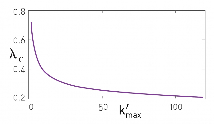
Image 10.22
Immunizing the Hubs
In heterogenous networks a virus can be eradicated by increasing the epidemic threshold through hub immunization. The figure shows the expected epidemic threshold if we immunize all nodes with degree larger than k'max. The more hubs are immunized (i.e. the smaller is k'max), the larger is λc, increasing the chance that the disease dies out. Immunizing the hubs changes the network on which the disease spreads, making the hubs invisible to the pathogen (Image 10.23).
The hubs are responsible for the large variance of heterogenous networks. Therefore if we immunize the hubs, i.e. all nodes whose degree exceeds some preselected k'max, we decrease the variance and increase the epidemic threshold according to (10.26) [68,69]. Indeed, if nodes with degrees k>k'max are absent, the epidemic threshold changes to (ADVANCED TOPICS 10.C)
Therefore, for γ < 3, the more hubs we cure (i.e. the smaller is k'max), the larger will be the epidemic threshold (Image 10.22). By immunizing a sufficient fraction of the hubs we can drop λc below λ= β/µ that characterizes the pathogen. This procedure is equivalent with altering the underlying network: By immunizing the hubs, we are fragmenting the contact network, making more difficult for the pathogen to reach the nodes in other components (Image 10.23).
Image 10.23
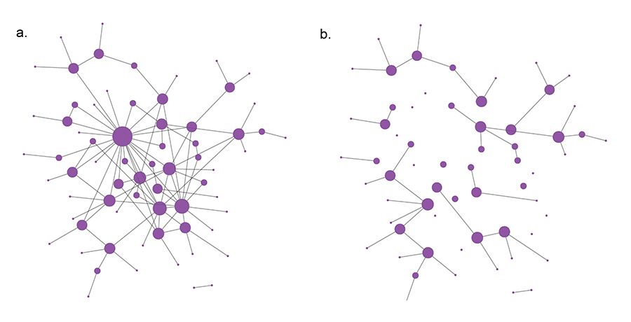
Robustness and Immunization
Scale-free networks show a remarkable resilience to random node and link failures (CHAPTER 8). At the same time, they are vulnerable to attacks: If we remove their most connected nodes, scale-free networks break apart. This phenomena has many similarities to the immunization problem: Random immunization is unable to eradicate a disease, but selective immunization, that targets the hubs, can restore a finite critical threshold, helping us eradicate the disease. The analogy is not accidental: The robustness and the immunization problem can be both linked to the diverging 〈k2〉. Indeed, the vanishing epidemic threshold is equivalent with the finding that the percolation threshold under random node removal problem converges to one (ADVANCED TOPICS 10.D). Similarly, the re-emergence of the epidemic threshold under hub immunization is equivalent with the small percolation threshold characterizing a scale-free network under attack. Therefore, the attack and targeted immunization problems represent two sides of the same coin.
To illustrate the equivalence between attacks and targeted immunization, consider the network shown in (a). An attack that removes its five largest hubs breaks the network into many isolated islands, as shown in (b). Targeted immunization plays the same role: By making the hubs immune to the disease, the network on which the pathogen spreads becomes the fragmented network in (b). As the immunized network is broken into small islands, the pathogen will be stuck in one of the small clusters, unable to infect the nodes in the other clusters.
Hub immunization represents a perspective change in immunization protocols: instead of trying to decrease the spreading rate using random immunization, we must alter the topology of the contact network, which in turn increases λc above the biologically determined λ= β/µ.
The problem with a hub-based immunization strategy is that for most epidemic processes we lack a detailed map of the contact network. Indeed, we do not know the number of sexual partners each individual has in a population, nor can we accurately identify the super-spreaders during an influenza outbreak. In other words it is difficult to identify the hubs. Yet, we can still exploit the network topology to design more efficient immunization strategies. To do so, we rely on the friendship paradox, the fact that on average the neighbors of a node have higher degree than the node itself (BOX 7.1). Therefore, by immunizing the acquaintances of a randomly selected individual, we target the hubs without having to know precisely which individuals are hubs. The procedure consists of the following steps [70]:
Choose randomly a p fraction of nodes, like we do during random immunization. Call these nodes Group 0.
Select randomly a link for each node in Group 0. We call Group 1 the set of nodes to which these links connect to. For example, we ask each individual from Group 0 to nominate one of its acquaintance with whom he/she engaged in an activity that could have resulted in the transmission of the pathogen. In the case of HIV, ask them to name a sexual partner.
Immunize the Group 1 individuals.
Image 10.24
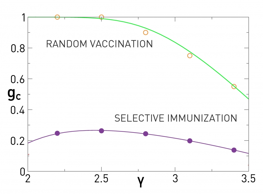
Selective Immunization of Scale-free Networks
The critical immunization threshold gc in function of the degree exponent γ of the contact network on which the pathogen spreads following the SIS model. The curves correspond to two immunization strategies: random immunization (green) and selective immunization (purple), that immunizes a first neighbor of a randomly selected node. The continuous lines represent the analytical results while the symbols represent simulation data for N=106 and m=1. As the population has a finite size, we have gc < 1 for random immunization even for γ < 3. Redrawn after [70].
This strategy requires no information about the global structure of the network. Yet, according to (7.3) the probability that a node with k links belongs to Group 1 is proportional to kpk. Consequently the Group 1 individuals have higher average degree than the Group 0 individuals. The implications of this bias are illustrated in Image 10.24, which shows the critical threshold required to eradicate a pathogen for a scale-free network with degree exponent γ. The figure offers several key insights:
Random Immunization
The top curve shows gc for random immunization. For heterogeneous networks (small γ) we find that gc ≈ 1, indicating that we must immunize all nodes to eradicate the disease. As γ approaches 3 the network develops a finite epidemic threshold and gc drops. Hence for large γ, immunizing a sufficiently high fraction of the population can eradicate the pathogen.
Selective Immunization
For the biased strategy gc is systematically under 30%. Therefore by immunizing a randomly chosen neighbor of 30% of the nodes, we could eradicate the disease. The efficiency of this strategy depends only weakly on γ. Selective immunization is more efficient than random immunization even for high γ, when hubs are less prominent.
Section 10.7
Epidemic Prediction
During much of its history humanity has been helpless when faced with a pandemic. Lacking drugs and vaccines, infectious diseases repeatedly swept through continents, decimating the world's population. The first vaccine was tested only in 1796 and the systematic development of vaccines and cures against new pathogens became possible only in the 1990s. Despite the spectacular medical advances, we have effective vaccines only against a small number of pathogens. Consequently transmission-reducing and quarantine-based measures remain the main tools of health professionals in combatting new pathogens. For the combination of vaccines, treatments and quarantine-based measures to be effective, we need to predict when and where the pathogen emerges next, allowing local health officials to best deploy their resources.
The real-time prediction of an epidemic outbreak is a very recent development. The ground was set by the development of the epidemic modeling framework in the 1980s [72] and by the 2003 SARS epidemic, which resulted in worldwide reporting guidelines about ongoing outbreaks. The subsequent systematic availability of data pertaining to a pandemic [1] offered real-time input to modeling efforts. The 2009 H1N1 outbreak was the first beneficiary of these developments, becoming the first pandemic whose spread was predicted in real time.
The emergence of any new pathogen raises several key questions:
Where did the pathogen originate?
Where do we expect new cases?
When will the epidemic arrive at various densely populated areas?
How many infections are to be expected?
What can we do to slow its spread?
How can we eradicate it?
Today these questions are addressed using powerful epidemic simulators that consider as input demographic, mobility-related (Video 10.4), and epidemiological data [73-75]. The algorithms behind these tools range from stochastic meta-population models [76-78] to agent-based computer simulations that capture the behavior and the interactions of millions of individuals [79]. In this section we summarize the capabilities of these tools, highlighting the role of network science in these developments.
Video 10.4 North American Flight Patterns
Real time flights across North America, relying on data released by the Federal Aviation Administration. This global transportation network is responsible for the spread of pathogens across continents. Consequently flight schedules represent the input for epidemic forecasts. While this video, produced by Aaron Koblin, could easily be seen as a purely scientific illustration, it is also viewed as digital art by the art community. Indeed, the video is now in Media Art collection of the Museum of Modern Art (MoMA) in New York.
Real-Time Forecast
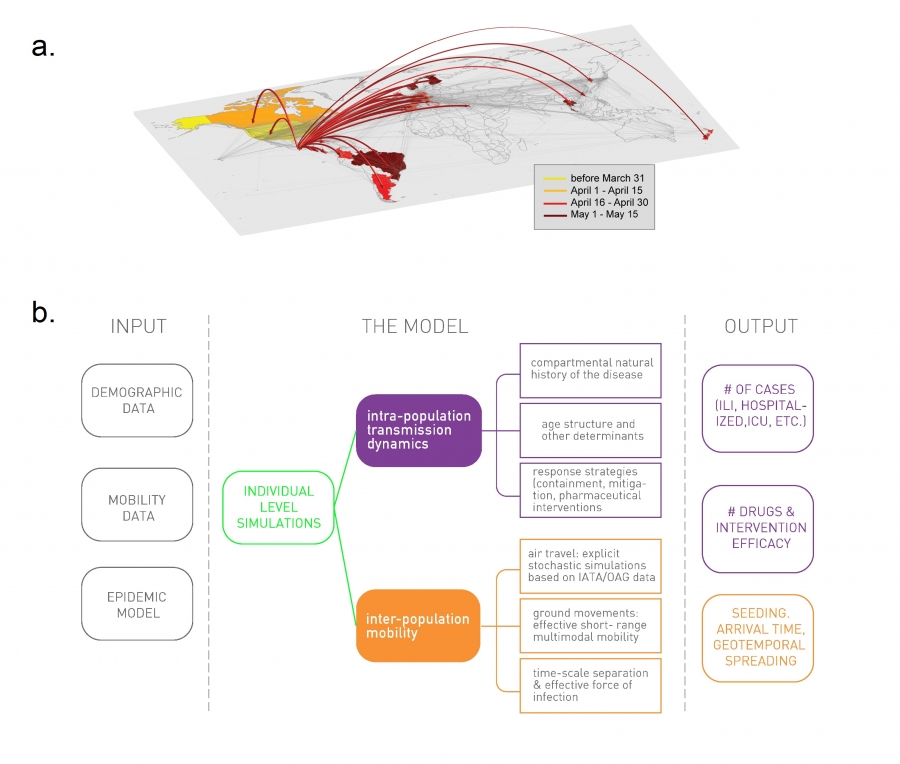
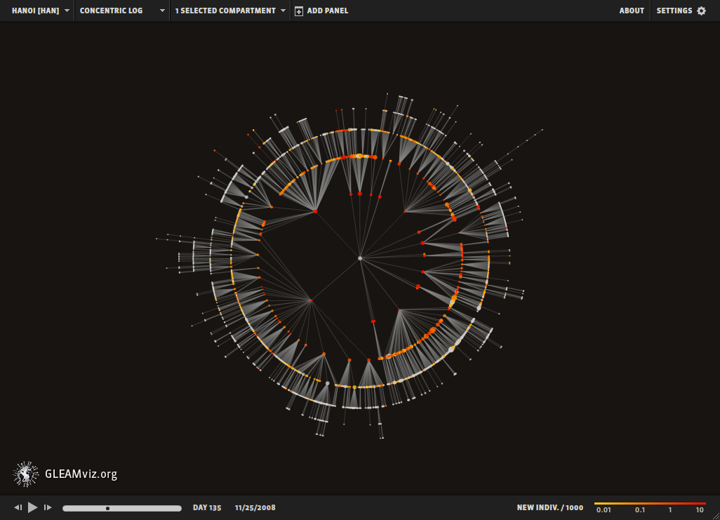
Epidemic forecast aims to foresee the real time spread of a pathogen, predicting the number of infected individuals expected each week in each major city [79,80]. The first successful real time pandemic forecast based on network science relied on the Global Epidemic and Mobility (GLEAM) computational model [80] (Image 10.26, Video 10.5), a stochastic framework that uses as input high-resolution data on worldwide human demography and mobility. GLEAM employs a network-based computational model:
GLEAM maps each geographic location into the nodes of a network.
Transport between these nodes, representing the links, are provided by global transportation data, like airline schedules (Video 10.4).
GLEAM estimates the epidemic parameters, like the transmission rate or reproduction number, using a network-based approach: It relies on chronological data that captures the worldwide spread of the pandemic, rather than medical reports [81].
Video 10.5 GLEAM
A video describing the GLEAM software package for epidemic prediction.
Image 10.26
Modeling the 2009 H1N1 Pandemic
The spread of the H1N1 virus during the early stage of the 2009 outbreak. The arrows represent the arrival of the first infections in previously unaffected countries. The color code indicates the time of the virus’ arrival.
The flowchart of the Global Epidemic and Mobility (GLEAM) computational model, used to predict the real-time spread of pathogens like H1N1 or Ebola. The left column (Input) represents the input databases, capturing demographic, mobility and epidemiological information. The center column (model) describes the network-based dynamic processes that are modeled at each time step. The right column (Output) offers examples of quantities the model can predict. After [82].
GLEAM then implements the network-based epidemic framework described in SECTION 10.3, generating a large number of potential outcomes of the pathogen’s global progression for the coming months. For H1N1 the predictions were compared with data collected from surveillance and virologic sources in 48 countries during the full course of the pandemic [80], resulting in several key findings:
Peak Time
Peak time corresponds to the week when most individuals are infected in a particular country. Predicting the peak time helps health officials decide the timing and the quantity of the vaccines or treatments they distribute. The peak time depends on the arrival time of the first infection and the demographic and the mobility characteristics of each country. The observed peak time fell within the prediction interval for 87% of the countries (Image 10.27). In the remaining cases the difference between the real and the predicted peak was at most two weeks.
Early Peak
GLEAM predicted that the H1N1 epidemic will peak out in November, rather than in January or February, the typical peak time of influenza-like viruses. This unexpected prediction turned out to be correct, confirming the model’s predictive power. The early peak time was a consequence of the fact that H1N1 originated in Mexico, rather than South Asia (where many flu viruses come from), hence it took the virus less time to arrive to the northern hemisphere.
The Impact of Vaccination
Several countries implemented vaccination campaigns to accelerate the decline of the pandemic. The simulations indicated that these mass vaccination campaigns had only negligible impact on the course of the epidemic. The reason is that the timing of these campaigns was guided by the expectation of a January peak time, prompting the deployment of the vaccines after the November 2009 peak [83], too late to have a strong effect.
Image 10.27
Activity Peaks for H1N1
The predicted and the observed peak time for the H1N1 virus in several countries. The peak time corresponds to the week when most individuals are infected by the pathogen, and is measured in weeks after the beginning of the epidemic. The model predictions were obtained by analyzing 2,000 stochastic realizations of the outbreak, generating the error bars in the figure. After [82].
‘What if’ Analysis
By incorporating the time and nature of each containment and mitigation procedure, simulations can estimate the efficiency of specific contingency plans [73-75,77,84]. Next we discuss the impact of two such interventions.
Travel Restrictions
Given the important role air travel plays in the spread of a pathogen, faced with a dangerous pandemic, like an Ebola outbreak (Image 10.28), the first instinct is to restrict travel. Yet, in a world where key resources travel by air, a travel ban leads to economic collapse. Therefore before resorting to a travel ban, we must make sure that travel restrictions have beneficial effects on the pandemic. For this we must realize that awareness of a viral outbreak results in self-imposed travel reductions. For example, there was a 40% decline in travel to and from Mexico in May 2009, during the H1N1 outbreak, as individuals canceled non-necessary business and leisure activities in the infected region. The modeling indicates [80,82] that this 40% reduction delayed the arrival of the first infection with less than 3 days in various countries around the world. Furthermore, even if travel dropped 90%, the peak time is delayed with less than 20 days (Image 10.29).
Most important, travel restrictions do not decrease the number of infected individuals. They only delay the outbreak, offering local authorities more time to prepare for the pandemic. Hence travel restrictions are effective only if the delay caused by them increases local vaccination levels or helps the deployment of cures.
Image 10.28
The Deadliest Outbreak
With a fatality rate in the vicinity of 80%, the Ebola virus is one of the deadliest viruses known to humans. Its first known incidence was in 1976 in Zaire, killing 280 of the 312 infected individuals by hemorrhagic fever, a combination of high fever and bleeding disorder. The virus can be transmitted by contact with the blood or the secretion of an infected individual.
Antiviral Treatment
During the 2009 H1N1 pandemic Canada, Germany, Hong Kong, Japan, the UK, and the USA distributed antiviral drugs to mitigate the impact of the disease [85]. This prompted modelers to ask what would have been the impact if all countries that had drug stockpiles would have distributed it to their population [86]. The simulations indicate that peak times would have been delayed with about 3 to 4 weeks, offering time to immunize a larger fraction of the population before the pandemic reached its peak.
Image 10.29
The Impact of Travel Reduction
The impact of travel reduction on the arrival time of the H1N1 virus from Mexico to various countries, compared with the reference scenario of no travel reduction. The percentages on the vertical axis show the degree of travel reduction implemented around the world. The largest delay is less than 20 days, observed for a 90% travel restriction. After [77].
Efective Distance
Before cars and airplanes pathogens traveled on foot or at most with the speed of a horse. Hence a pandemic like the Black Death in Europe moved slowly from village to village (Image 10.8), following a diffusive process described by simple reaction-diffusion models [87,88]. As the next infection always emerged in the geographic proximity of the previous infections, there was a strong correlation between the time of the outbreak and the physical distance from the origin of the outbreak.
Today, with airline travel, physical distance has lost its relevance for epidemic phenomena. A pathogen that emerges in Manhattan can just as easily travel to London than to Garrison, NY, a village an our drive from Manhattan. This prompts us to ask: Is there a better space to view the spread of an epidemic than the physical space? Such space does exist if we replace the conventional geographic distance with an effective distance derived from the mobility network [89]. The nodes of the mobility network are cities and the links represent the amount of travel between them. Each link is directed and weighted, characterized by a flux-fraction 0 ≤ pij ≤ 1, that represents the fraction of travelers that leave node i and arrive at node j. The values of pij can be extracted from airline schedules, having pij > 0 only if there is direct travel from i to j.
Given the multiple routes a person can take between any two cities, a pathogen can follow multiple paths on the mobility network. Yet, its spread is dominated by the most probable trajectories predicted by the mobility matrix pij. This allows us to define the effective distancedij between two connected locations i and j, as
If pij is small, implying that only a small fraction of individuals that leave from i travel to j, then the effective distance between i and j is large. Note that dij ≠ dij: For a small village i located near a metropolis j we expect dij to be small, as most travelers from i go to j. Yet, dij is large as only a small fraction of travelers leaving the metropolis head to the small village. The logarithm in (10.31) accounts for the fact that effective distances are additive, whereas probabilities along multi-step paths are multiplicative.
The spread of a pathogen, as predicted by GLEAM, from three initial outbreak locations. While the geographic spreading pattern is difficult to interpret, in the effective distance representation the pandemic follows a regular radial pattern (Image 10.31).
The observed spreading patterns prompt us to ask: What is the speed of a typical pathogen as it spreads around the globe? The speed depends on three key parameters:
The basic reporduction number R0, which is in the vicinity of 2 for influenza type viruses (Table 10.2).
The recovery rate, which is approximately 3 days for influenza.
The mobility rate, which represents the total fraction of the population that travels during a day. This parameter is in the range of 0.01-0.001.
Running GLEAM (Image 10.26) with these parameters we can compute the correlation between the arrival time and the geographic distance to the source of the epidemic, obtaining a speed of about 250-300 km/day. Therefore an influenza virus moves through a continent with the speed of a sports car or of a smaller airplane [89].
As Image 10.31 indicates (see also Online Resource 10.6), if we use (10.31) to represent the distance of each city from the source of an epidemic, the pathogen follows circular wave fronts. This is in contrast with the complex spreading pattern we observe if we view the pandemic in the geographical space. Furthermore, while the arrival time of H1N1 appears to be random if plotted in function of the physical distance, it correlates strongly with the effective distance (Image 10.32). We can therefore use the effective distance to determine the speed of a pathogen (Online Resource 10.6).
A surprising but welcome aspect of epidemic forecast is that the predictions of different models are rather similar, despite the fact that they use different mobility data (airline schedules [25,26] or dollar bill movement [24]) and different assumptions about the epidemic parameters (recovery rate, transmission rate, etc). The effective distance helps us understand why the various model predictions converge. Indeed, we can write the arrival time of a pathogen to location a as [89]
Therefore the arrival time is the ratio of the effective distance deff and an effective speed Veff. The effective speed is determined only by the epidemiological parameters of the pathogen, whereas the effective distance deff depends only on the topology of the mobility network encoded by pij. When confronted with a new outbreak, the pathogen-specific epidemiological parameters are unknown in the beginning. However, (10.32) predicts that the relative arrival times are independent of the epidemiological parameters. For example, for an outbreak that starts at node i, the ratio of the arrival times to nodes j and l is
i.e. the ratio depends only on the effective distances. Therefore, the relative arrival times of the disease depend only on the topology of the mobility network. As the mobility patterns around the world are unique and model-independent, the predictions of different models converge, independent of the choice of the epidemiological parameters.
Image 10.31
Effective Distance
The spread of a pandemic with an initial outbreak in Hong Kong. Regions with a large number of infections are shown as red nodes. Each panel compares the state of the system in the conventional geographic representation (bottom) with the effective distance representation (top). The complex spatial pattern observed in the geographic representation becomes a circular wave that moves outwards at constant speed in the effective distance representation (see also the Online Resource 10.6). After [89].
In summary, joint advances in data collection and network epidemics have offered the capability to predict the real-time spread of a pathogen. The developed models can help design response and mitigation scenarios, train health and emergency personnel, can be used to explore the impact of various interventions, from quarantine to travel restrictions, and to optimize the deployment of treatments and vaccines.
Interestingly, the recent success of epidemic forecast is not due to the improved understanding of the underlying biology of infectious pathogens. It can be attributed instead to the lucky situation that when it comes to the spreading of a pathogen, the epidemic parameters are of secondary importance. The most important factor is the structure of the mobility network. That, however, can be accurately estimated from travel schedules, allowing us to turn human mobility patterns into accurate predictions about the course of a pandemic.
Image 10.32
Effective Distance and Arrival Time
Geographic Distance
Arrival times vs. geographic distance from its source (Mexico) for the 2009 H1N1 pandemic. Each circle represents one of the 140 affected countries and the symbol size indicates the total traffic in each country. Arrival times are the date of the first confirmed case in a given country after the beginning of the outbreak on March 17, 2009. In this representation the arrival time and the geographic distance are largely independent of each other (R0=0.0394).
Effective Distance
Epidemic arrival time Ta vs. effective distance Deff for H1N1, demonstrating the strong correlations between the effective distance (10.31) and the arrival time. After [89].
Section 10.8
Summary
Most networks facilitate transfer along their links: transfer of trust, knowledge, habits or information (social networks), electricity (power grid), money (financial networks), goods (trade networks). To understand these phenomena, we must understand how the network topology affects these dynamical processes. In this chapter we focused on the spread of pathogens along the links of the network, the area where our understanding of the interplay between dynamical phenomena and network topology is the most advanced. We showed that the network topology has a drastic impact on the dynamics of the spreading process, offering distinct predictions for spreading on random and on scale-free networks. This finding laid the ground for addressing a wider class of problems: the need to systematically understand the impact networks have on various dynamical processes [100], an increasingly active chapter of network science [101,102].
Modeling the spread of pathogens also represents an important practical application of network science. The advances in this area were rather spectacular, giving birth to accurate epidemic forecasts, something that was only a dream a decade earlier. Two advances made this possible. The first is the emergence of a robust theoretical framework to describe network-based epidemics. The second is access to accurate real time data on human travel and demographics, allowing us to reconstruct the mobility network that is responsible for the global spread of a pathogen. As we have seen in SECTION 10.7, the biological parameters and the network contributions to the accuracy of the observed predictive power are decoupled. Consequently, an accurate forecast requires primarily an accurate knowledge of the mobility network.
The analytical framework of network epidemics has offered a number of unexpected results, the most important being the vanishing characteristic spreading time and epidemic threshold in heterogeneous networks. As most contact networks encountered in epidemic processes have a broad degree distribution, these results are of immediate and of lasting theoretical and practical interest.
Equally important are the insights network epidemiology offers for immunization strategies. As we showed in SECTION 10.6, while random immunization can successfully eradicate a virus that spreads on a random network, this strategy is suboptimal in a scale-free network. As most contact networks are heterogenous, this is a rather depressing conclusion. Yet, we showed that selective immunization strategies can restore the epidemic threshold and suppress the prevalence of a pathogen. Selective immuniztion succeeds by systematically altering the topology of the network on which a pathogen spreads.
Section 10.9
Homework
Epidemics on Networks
Calculate the characteristic time τ and the epidemic threshold λc of the SI, SIS and SIR models for networks with
Exponential degree distribution.
Stretched exponential degree distribution.
Delta distribution (all nodes have the same degree)
Assume that the networks are uncorrelated and infinite. Refer to Table 4.2 for the functional form of the distribution and the corresponding first and second moments.
Random Obesity in Social Networks
Consider a social network with degree distribution pk, where 50% of the nodes are obese. Make the assumption that obese nodes are distributed randomly within the network.
If the network has degree correlation, encoded in the join probability ekk', what is the probability P(øo) that a non-obese (ø) individual is friend with an obese individual (o)? And what is the probability P(oo) that two obese individuals are friends?
Assume that the network is uncorrelated. How many second neighbors of a degree-k node are obese?
Calculate the same quantities of (a)-(b) if the percentage of obese increases to 70%.
Immunization
Choose four networks from Table 4.1 (assume that directed networks behave like undirected and uncorrelated networks with pk = pkin ) and consider an epidemic process spreading on them. Remember: not only pathogens, but also ideas or opinions can spread on a network! Determine for each network the critical fraction gc necessary to stop the epidemic if we randomly immunise a g-fracion of the nodes. How would the epidemic threshold λc change if all nodes with degree higher than 1,000 are immunized?
Epidemic on Bipartite Networks
Consider a bipartite network, with two types of nodes, which we indicate as male (M) and female (F).On this network a pathogen can be transmitted only from the node of one set to the node of the other set. Assume that the rate of transmission from an M node to an F node, βM→F , is different from the rate of transmission from an F node to an M node, βF→M . Write the equations of the corresponding SI model, assuming the degree block approximation and that the network is uncorrelated.
Section 10.10
Advanced Topic 10.A Microscopic Models of Epidemic Processes
In SECTIONS 10.2 and 10.3 we relied on the continuum approach to describe epidemic phenomena. In this section we show that the key results can be derived using microscopic models and probability-based reasoning. These arguments help us understand the origin of the continuum approach and improve our understanding of epidemic phenomena.
Deriving the Epidemic Equation
We start by deriving the continuum model (10.3) from the microscopic processes that describe the interactions between two individuals [101]. Consider a susceptible individual in contact with an infected individual, so that the susceptible individual becomes infected with probability βdt during the time interval dt. The probability that the susceptible individual is not infected in the dt interval is (1– βdt). If the susceptible individual i has degree ki, each of its ki links could in principle infect it. Therefore the probability that it avoids infection is (1– βdt)ki. Finally the total probability that node i becomes infected in time dt is 1– (1– βdt)ki, or one minus the total probability that it is not infected. Assuming βdt ≪ 1, at the leading order the probability that a susceptible individual becomes infected is
In a random network all nodes have approximately 〈k〉 neighbors. Replacing ki with 〈k〉 in (10.33) we obtain the first term of the continuum equation (10.3). If we do not replace ki with 〈k〉, we obtain to the first term of (10.13), capturing the spread of a pathogen in a heterogenous network
Epidemic Threshold and Network Topology
A key result of SECTION 10.3 connects the network topology to the epidemic threshold λc, a result derived using the continuum theory. We can arrive at the same result using a mechanistic argument that illustrates the connection between the epidemic threshold and the network topology.
Consider a pathogen that is transmitted with probability β in a unit time. Therefore in a unit time an infected node with degree k will infect βk neighbors. If each infected node recovers at rate µ, then the characteristic time that a node stays infected is 1/µ. The pathogen can persist in the population only if during this 1/µ time interval the infected node infects at least one other node. Otherwise, the pathogen gradually dies out.
In other words, if βk/µ < 1, then our degree-k node recovers before it could infect other nodes. If we consider a random network, where most nodes have comparable degrees, k~〈k〉, the condition βk/µ=1 allows us to calculate the epidemic threshold. Using λ= β/µ we obtain λc =1/〈k〉, which is the high-k limit of the result (10.25) derived for random networks. It tells us that the ability of a pathogen to spread is determined by the interplay between the epidemiological characteristics of the pathogen (β and µ) and the network topology (〈k〉).
In a scale-free network nodes have widely different degrees. Therefore while the network’s average degree may satisfy β〈k〉/µ < 1, suggesting that the virus will die out, for all nodes with k > 〈k〉 we have βk/µ > 1. If such a high degree node is infected, even if the spreading rate λ is under the threshold 1/〈k〉, the disease can spread, persisting in the hubs. This is the reason why the epidemic threshold vanishes in networks with high 〈k2〉.
Section 10.11
Advanced Topic 10.B Analytical Solution of the SI, SIS and SIR Models
In this section we solve the SI, SIS and SIR models on a network, deriving the results summarized in Table 10.3, namely the characteristic spreading time τ and the epidemic threshold λc for each model.
The Density Function
The density function Θk provides the fraction of infected nodes in the neighborhood of a susceptible node with degree k. As discussed in SECTION 10.3, to calculate ik, we must first determine Θk. If a network lacks degree correlations, the probability that a link points from a node with degree k to a node with degree k' is independent of k. Hence the probability that a randomly chosen link points to a node with degree k' is the excess degree (7.3),
At least one link of each infected node is connected to another infected node, the one that transmitted the infection. Therefore the number of links available for future transmission is (k'–1), allowing us to write
In other words, in the absence of degree correlations Θk is independent of k. Differentiating (10.34) we obtain
To make further progress, we need to consider the specific model the pathogen follows.
SI Model
Using (10.13) and (10.35) we obtain
To predict the early behavior of the epidemics, we consider the fact that for small t the fraction of infected individuals is much smaller than one. Therefore we can neglect the second order terms in (10.36), obtaining
This has the solution
where
Using the initial condition
which means that initially an i0 fraction of nodes are infected uniformly (hence ik(t=0)=i0 for all k), we obtain the time dependent Θ as
We insert this into (10.13) to arrive at (10.15).
SIR Model
In the SIR model the density of infected nodes follows
where rk is the fraction of recovered nodes with degree k. Keeping only the first order terms (which means that we ignore ik and rk in the parenthesis above, as for small t they are much smaller than one), we obtain
Multiplying this equation with (k–1)pk/〈k〉 and summing over k we have
The solution of (10.43) is
where the characteristic time for the SIR model is
A global outbreak is possible only if τ > 0, i.e. when the number of infected nodes grows exponentially with time. This yields the condition for a global outbreak as
allowing us to write the epidemic threshold for the SIR model as (Table 10.3)
SIS Model
In the SIS model the density of infected nodes is given by (10.18),
There is a small but important difference in the density function of the SIS model. For the SI and the SIR models, if a node is infected, then at least one of its neighbors must also be infected or recovered, hence at most (k–1) of its neighbors are susceptible, the origin of the (-1) term in the paranthesis of (10.34) . However, in the SIS model the previously infected neighbor can become susceptible again, therefore all k links of a node can be available to spread the disease. Hence we modify the definition (10.34) to obtain
Again keeping only the first order terms we obtain
Multiplying the equation with (k–1)pk/〈k〉 and summing over k we have
This again has the solution
where the characteristic time of the SIS model is
A global outbreak is possible if τ>0, which yields the condition for a global outbreak as
and the epidemic threshold for the SIS model as (Table 10.3)
In this section we derive the epidemic threshold for the SIS and SIR models on scale-free networks under hub immunization. We start with an uncorrelated network with power law degree distribution pk=c.k-γ where c≈(γ–1)/kmin-γ+1 and k ≥ kmin. In SECTION 10.16 we obtained for the critical spreading rate,
and
Under hub immunization we immunize all nodes whose degree is larger than k0. From the perspective of the epidemic this is equivalent with removing the high degree nodes from the network. Therefore to calculate the new critical spreading rate, we need to determine the average degree 〈k'〉 and the second moment 〈k'2〉 after the hubs have been removed. This problem was addressed in the ADVANCED TOPICS 8.F, where we studied the robustness of a network under attack. We have seen that hub removal has two effects:
The maximum degree of the network changes to k0.
The links connected to the removed hubs are also removed, as if we randomly remove an
fraction of links.
The degree distribution of the resulting network is
According to (8.39) and (8.40) this yields
where 〈k〉 is the average and 〈k2〉 is the second moment of the degree distribution before the link removal, but with maximum degree k0. For the SIS model this means
where, according to equation (8.47), for 2 > γ > 3
Combining (10.56), (10.57) and (10.58) we obtain
For the SIR model a similar calculation yields
For both the SIR and SIS models if k0 ≫ kmin we have
Section 10.13
Advanced Topic 10.D The SIR Model and Bond Percolation
The SIR model is a dynamical model that captures the time dependent spread of an infection in a network. Yet, it can be mapped into a static bond percolation problem [103-106]. This mapping offers analytical tools that help us predict the model’s behavior.
Consider an epidemic process on a network, so that each infected node transmits a pathogen to each of its neighbors with rate β, and recovers after a recovery time τ=1/µ. We view the infection as a Poisson process, consisting of series of random contacts with average interevent time βτ. Therefore the probability that an infected node does not transmit the pathogen to susceptible neighbors decreases exponentially in time, or e–βτ. The infected node stays infected until it recovers in τ=1/µ time. Therefore the overall probability that the pathogen is passed on is 1–e–βτ.
This process is equivalent with bond percolation on the same network, where each directed link is occupied with probability pb=1–e–βτ (Image 10.35). If β and τ are the same for each node, the network can be considered undirected. Although this mapping looses the temporal dynamics of the epidemic process, it has several advantages:
The total fraction of infected nodes in the endemic state maps into the size of the giant component of the percolation problem.
The probability that a pathogen dies out before reaching the endemic state equals the fraction of the nodes in a randomly selected finite component in the percolation problem.
We can determine the epidemic threshold by exploiting the known properties of bond percolation. Consider the average number of links outgoing from a node that can be reached by a link. This allows us to retrace the course of the epidemic: If an infected individual infects on average at least one other individual, then the epidemic can reach an endemic state. Since a node can be reached by one of its k links, the probability to be reached is kpk/N〈k〉. The probability of each of its k–1 outgoing links infecting its neighbor is pb.
Image 10.36
Mapping Epidemics into Percolation
Consider the contact network on which the epidemic spreads. To map the spreading process into percolation, we leave in place each link with probability, pb=1–e–β/μ, a probability determined by the biological characteristics of the pathogen. Therefore links are removed with probability e–β/μ. The cluster size distribution of the remaining network can be mapped exactly into the outbreak size. For large β/μ we will likely have a giant component, indicating that we could face a global outbreak. β/μ corresponds to a virus that has difficulty spreading and we end up with numerous small clusters, indicating that the pathogen will likely die out.
Since the network is randomly connected, as long as the epidemic has not spread yet, the average number of neighbors infected by the selected node is
An endemic state can be reached only if 〈Ri〉 > 1, obtaining the condition for the epidemic as [107,108]
Equation (10.62) agrees with the result (10.46) derived earlier from the dynamical models: Scale-free networks with γ ≤ 3 have a divergent second moment, hence such networks undergo a percolation transition even at pb→0. That is, a virus can spread on this network regardless of how small is the infection probability β or how small is the recovery time τ.
Section 8.14
Bibliography
[1] D. Normile. The Metropole, Superspreaders and Other Mysteries. Science, 339:1272-1273, 2013.
[2] J.O. Lloyd-Smith, S.J. Schreiber, P.E. Kopp, and W.M. Getz. Superspreading and the effect of individual variation on disease emergence. Nature, 438:355-359, 2005.
[3] M. Hypponen. Malware Goes Mobile. Scientific American, 295:70, 2006.
[4] P. Wang, M. Gonzalez, C. A. Hidalgo, and A.-L. Barabási. Understanding the spreading patterns of mobile phone viruses. Science, 324:1071- 1076, 2009.
[5] E.M. Rogers. Diffusion of Innovations. Free Press, 2003.
[6] T.W. Valente. Network models of the diffusion of innovations. Hampton Press, Cresskill, NJ, 1995.
[7] History and Epidemiology of Global Smallpox Eradication From the training course titled "Smallpox: Disease, Prevention, and Intervention". The CDC and the World Health Organization. Slides 16-17.
[8] R.M. Anderson and R.M. May. Infectious Diseases of Humans: Dynamics and Control. Oxford University Press, Oxford, 1992.
[9] R. Pastor-Satorras and A. Vespignani. Epidemic spreading in scalefree networks. Physical Review Letters, 86:3200–3203, 2001.
[10] R. Pastor-Satorras and A. Vespignani. Epidemic dynamics and endemic states in complex networks. Physical Review E, 63:066117, 2001.
[11] Y. Wang, D. Chakrabarti, C, Wang, and C. Faloutsos. Epidemic spreading in real networks: an eigenvalue viewpoint. Proceedings of 22nd International Symposium on Reliable Distributed Systems, pg. 25-34, 2003.
[12] R. Durrett. Some features of the spread of epidemics and information on a random graph. PNAS, 107:4491-4498, 2010.
[13] S. Chatterjee and R. Durrett. Contact processes on random graphs with power law degree distributions have critical value 0. Ann. Probab., 37: 2332-2356, 2009.
[14] C Castellano, and R Pastor-Satorras. Thresholds for epidemic spreading in networks. Physical Review Letters, 105:218701, 2010.
[15] B. Lewin. (ed.), Sex i Sverige. Om sexuallivet i Sverige 1996 [Sex in Sweden. On the Sexual Life in Sweden 1996]. National Institute of Public Health, Stockholm, 1998.
[16] F. Liljeros, C. R. Edling, L. A. N. Amaral, H. E. Stanley, and Y. Åberg. The web of human sexual contacts. Nature, 411:907-8, 2001.
[17] A. Schneeberger, C. H. Mercer, S. A. Gregson, N. M. Ferguson, C. A. Nyamukapa, R. M. Anderson, A. M. Johnson, and G. P. Garnett. Scale-free networks and sexually transmitted diseases: a description of observed patterns of sexual contacts in Britain and Zimbabwe. Sexually Transmitted Diseases, 31: 380-387, 2004.
[18] W. Chamberlain. A View from Above. Villard Books, New York, 1991.
[19] R. Shilts. And the Band Played On. St. Martin’s Press, New York, 2000.
[20] P. S. Bearman, J. Moody, and K. Stovel. Chains of affection: the structure of adolescent romantic and sexual networks. Am J Sociol., 110:44-91, 2004.
[21] M. C. González, C. A. Hidalgo, and A.-L. Barabási. Understanding individual human mobility patterns. Nature, 453:779-782, 2008.
[22] C. Song, Z. Qu, N. Blumm, and A.-L. Barabási. Limits of Predictability in Human Mobility. Science, 327:1018-1021, 2010.
[23] F. Simini, M. González, A. Maritan, and A.-L. Barabási. A universal model for mobility and migration patterns. Nature, 484:96-100, 2012.
[24] D. Brockmann, L. Hufnagel, and T. Geisel. The scaling laws of human travel. Nature, 439:462–465, 2006.
[25] V. Colizza, A. Barrat, M. Barthelemy, and A. Vespignani. The role of the airline transportation network in the prediction and predictability of global epidemics. PNAS, 103:2015, 2006.
[26] L. Hufnagel, D. Brockmann, and T. Geisel. Forecast and control of epidemics in a globalized world. PNAS, 101:15124, 2004.
[27] R. Guimerà, S. Mossa, A. Turtschi, and L. A. N. Amaral. The worldwide air transportation network: Anomalous centrality, community structure, and cities' global roles. PNAS, 102:7794, 2005.
[28] C. Cattuto, et al. Dynamics of Person-to-Person Interactions from Distributed RFID Sensor Networks. PLoS ONE, 5:e11596, 2010.
[29] L. Isella, C. Cattuto, W. Van den Broeck, J. Stehle, A. Barrat, and J.-F. Pinton. What’s in a crowd? Analysis of face-to-face behavioral networks. Journal of Theoretical Biology, 271:166-180, 2011.
[30] K. Zhao, J. Stehle, G. Bianconi, and A. Barrat. Social network dynamics of face-to-face interactions. Physical Review E, 83:056109, 2011.
[31] J. Stehlé, N. Voirin, A. Barrat, C Cattuto, L. Isella, J-F. Pinton, M. Quaggiotto, W. Van den Broeck, C. Régis, B. Lina, and P. Vanhems. High-resolution measurements of face-to-face contact patterns in a primary school. PLoS ONE, 6:e23176, 2011.
[32] B.N. Waber, D. Olguin, T. Kim, and A. Pentland. Understanding Organizational Behavior with Wearable Sensing Technology. Academy of Management Annual Meeting. Anaheim, CA. August, 2008.
[33] L. Wu, B.N. Waber, S. Aral, E. Brynjolfsson, and A. Pentland. Mining Face-to-Face Interaction Networks using Sociometric Badges: Predicting Productivity in an IT Configuration Task. In Proceedings of the International Conference on Information Systems. Paris, France. December 14-17 2008.
[34] M. Salathé, M. Kazandjievab, J.W. Leeb, P. Levisb, M.W. Feldmana, and J.H. Jones. A high-resolution human contact network for infectious disease transmission. PNAS, 107:22020–22025, 2010.
[35] A.-L. Barabási. The origin of bursts and heavy tails in human dynamics. Nature, 435:207-11, 2005.
[36] V. Sekara, and S. Lehmann. Application of network properties and signal strength to identify face-to-face links in an electronic dataset. Proceedings of CoRR, 2014.
[37] S. Eubank, H. Guclu, V.S.A. Kumar, M.V. Marathe, A. Srinivasan, Z. Toroczkai, and N. Wang. Modelling disease outbreaks in realistic urban social networks. Nature, 429:180-184, 2004.
[38] H. Ebel, L-I. Mielsch, and S. Bornholdt. Scale-free topology of e-mail networks. Physical Review E, 66:035103, 2002.
[39] M. Morris, and M. Kretzschmar. Concurrent partnerships and transmission dynamics in networks. Social Networks, 17:299-318, 1995.
[40] N. Masuda and P. Holme. Predicting and controlling infectious diseases epidemics using temporal networks. F1000 Prime Rep., 5:6, 2013.
[41] P. Holme, and J. Saramäki. Temporal networks. Physics Reports, 519:97-125, 2012.
[42] M. Karsai, M. Kivelä, R. K. Pan, K. Kaski, J. Kertész, A.-L. Barabási, and J. Saramäki. Small but slow world: how network topology and burstiness slow down spreading. Physical Review E, 83:025102(R), 2011.
[43] A. Vazquez, B. Rácz, A. Lukács, and A.-L. Barabási. Impact of non- Poissonian activity patterns on spreading processes. Physical Review Letters, 98:158702, 2007.
[44] A. Vázquez, J.G. Oliveira, Z. Dezsö, K.-I. Goh, I. Kondor, and A.-L. Barabási. Modeling bursts and heavy tails in human dynamics. Physical Review E, 73:036127, 2006.
[45] A.V. Goltsev, S.N. Dorogovtsev, and J.F.F. Mendes. Percolation on correlated networks. Physical Review E., 78:051105, 2008.
[46] P. Van Mieghem, H. Wang, X. Ge, S. Tang and F. A. Kuipers. Influence of assortativity and degree-preserving rewiring on the spectra of networks. The European Physical Journal B, 76:643, 2010.
[47] M. Boguná, R. Pastor-Satorras, and A. Vespignani. Absence of epidemic threshold in scale-free networks with degree correlations. Physical Review Letters, 90:028701, 2003.
[48] Y. Moreno, J. B. Gómez, and A.F. Pacheco. Epidemic incidence in correlated complex networks. Physical Review E, 68:035103, 2003.
[49] J.-P. Onnela, J. Saramaki, J. Hyvonen, G. Szabó, D. Lazer, K. Kaski, J. Kertész, and A.-L. Barabási. Structure and tie strengths in mobile communication networks. PNAS, 104:7332, 2007.
[50] M. S. Granovetter. The strength of weak ties. American Journal of Sociology, 78:1360–1379, 1973.
[51] A. Galstyan, and P. Cohen. Cascading dynamics in modular networks. Physical Review E, 75:036109, 2007.
[52] J. P. Gleeson. Cascades on correlated and modular random networks. Physical Review E, 77:046117, 2008.
[53] P. A. Grabowicz, J. J. Ramasco, E. Moro, J. M. Pujol, and V. M. Eguiluz. Social features of online networks: The strength of intermediary ties in online social media. PLOS ONE, 7:e29358, 2012.
[54] L. Weng, F. Menczer and Y.-Y. Ahn. Virality Prediction and Community Structure in Social Networks. Scientific Reports, 3:2522, 2013.
[55] S. Aral, and D. Walker. Creating social contagion through viral product design: A randomized trial of peer influence in networks. Management Science, 57:1623–1639, 2011.
[56] J. Leskovec, L. Adamic, and B. Huberman. The dynamics of viral marketing. ACM Trans. Web, 1, 2007.
[57] L. Weng, A Flammini, A. Vespignani, and F. Menczer. Competition among memes in a world with limited attention. Scientific Reports, 2:335, 2012.
[58] J. Berger, and K. L. Milkman. What makes online content viral? Journal of Marketing Research, 49:192–205, 2009.
[59] S. Jamali, and H. Rangwala. Digging digg: Comment mining, popularity prediction and social network analysis. Proc. Intl. Conf. on Web Information Systems and Mining (WISM), 32–38, 2009.
[60] G. Szabó and, B. A. Huberman. Predicting the popularity of online content. Communications of the ACM, 53:80–88, 2010.
[61] B. Suh, L. Hong, P. Pirolli, and E. H. Chi. Want to be retweeted? Large scale analytics on factors impacting retweet in twitter network. Proc. IEEE Intl. Conf. on Social Computing, 177–184, 2010.
[62] D. Centola. The spread of behavior in an online social network experiment. Science, 329:1194–1197, 2010.
[63] L. Backstrom, D. Huttenlocher, J. Kleinberg, and X. Lan. Group formation in large social networks: membership, growth, and evolution. Proc. ACM SIGKDD Intl. Conf. on Knowledge discovery and data mining, 44–54, 2006.
[64] M. Granovetter. Threshold Models of Collective Behavior. American Journal of Sociology, 83:1420–1443, 1978.
[65] N.A. Christakis, and J.H. Fowler. The Spread of Obesity in a Large Social Network Over 32 Years. New England Journal of Medicine, 35:370-379, 2007.
[66] N. A. Christakis and J. H. Fowler. The collective dynamics of smoking in a large social network. New England Journal of Medicine, 358:2249-2258, 2008.
[67] R. Pastor-Satorras, and A. Vespignani. Evolution and structure of the Internet: A statistical physics approach. Cambridge University Press, Cambridge, 2007.
[68] Z. Dezső and A-L. Barabási. Halting viruses in scale-free networks. Physical Review E, 65:055103, 2002.
[69] R. Pastor-Satorras and A. Vespignani. Immunization of complex networks. Physical Review E, 65:036104, 2002.
[70] R. Cohen, S. Havlin, and D. ben-Avraham. Efficient Immunization Strategies for Computer Networks and Populations. Physical Review Letters, 91:247901, 2003.
[71] F. Fenner et al. Smallpox and its Eradication. WHO, Geneva, 1988. http://www.who.int/features/2010/smallpox/en/
[72] L. A. Rvachev, and I. M. Longini Jr. A mathematical model for the global spread of influenza. Mathematical Biosciences, 75:3-22, 1985.
[73] A. Flahault, E. Vergu, L. Coudeville, and R. Grais. Strategies for containing a global influenza pandemic. Vaccine, 24:6751-6755, 2006.
[74] I. M. Longini Jr, M. E. Halloran, A. Nizam, and Y. Yang. Containing pandemic influenza with antiviral agents. Am. J. Epidemiol., 159:623-633, 2004.
[75] I.M. Longini Jr, A. Nizam, S. Xu, K. Ungchusak, W. Hanshaoworakul, D. Cummings, and M. Halloran. Containing pandemic influenza at the source. Science, 309:1083-1087, 2005.
[76] V. Colizza, A. Barrat, M. Barthélemy, A.-J. Valleron, and A. Vespignani. Modeling the world-wide spread of pandemic influenza: baseline case and containment interventions. PLoS Med, 4:e13, 2007.
[77] T. D. Hollingsworth, N.M. Ferguson, and R.M. Anderson. Will travel restrictions control the International spread of pandemic influenza? Nature Med., 12:497-499, 2006.
[78] C.T. Bauch, J.O. Lloyd-Smith, M.P. Coffee, and A.P. Galvani. Dynamically modeling SARS and other newly emerging respiratory illnesses: past, present, and future. Epidemiology, 16:791-801, 2005.
[79] I. M. Hall, R. Gani, H.E. Hughes, and S. Leach. Real-time epidemic forecasting for pandemic influenza. Epidemiol Infect., 135:372-385, 2007.
[80] M. Tizzoni, P. Bajardi, C. Poletto, J. J. Ramasco, D. Balcan, B. Gonçalves, N. Perra, V. Colizza, and A. Vespignani. Real-time numerical forecast of global epidemic spreading: case study of 2009 A/H1N1pdm. BMC Medicine, 10:165, 2012.
[81] D. Balcan, H. Hu, B. Gonçalves, P. Bajardi, C. Poletto, J. J. Ramasco, D. Paolotti, N. Perra, M. Tizzoni, W. Van den Broeck, V. Colizza, and A. Vespignani. Seasonal transmission potential and activity peaks of the new influenza A/H1N1: a Monte Carlo likelihood analysis based on human mobility. BMC Med., 7:45, 2009.
[82] P. Bajardi, et al. Human Mobility Networks, Travel Restrictions, and the Global Spread of 2009 H1N1 Pandemic. PLoS ONE, 6:e16591, 2011.
[83] P.Bajardi, C. Poletto, D. Balcan, H. Hu, B. Gonçalves, J. J. Ramasco, D. Paolotti, N. Perra, M. Tizzoni, W. Van den Broeck, V. Colizza, and A. Vespignani. Modeling vaccination campaigns and the Fall/Winter 2009 activity of the new A/H1N1 influenza in the Northern Hemisphere. EHT Journal, 2:e11, 2009.
[84] M.E. Halloran, N.M. Ferguson, S. Eubank, I.M. Longini, D.A.T. Cummings, B. Lewis, S. Xu, C. Fraser, A. Vullikanti, T.C. Germann, D. Wagener, R. Beckman, K. Kadau, C. Macken, D.S. Burke, and P. Cooley. Modeling targeted layered containment of an influenza pandemic in the United States. PNAS, 105:4639-44, 2008.
[85] G. M. Leung, A. Nicoll. Reflections on Pandemic (H1N1) 2009 and the international response. PLoS Med, 7:e1000346, 2010.
[86] A.C. Singer, et al. Meeting report: risk assessment of Tamiflu use under pandemic conditions. Environ Health Perspect., 116:1563-1567, 2008.
[87] R. Fisher. The wave of advance of advantageous genes. Ann. Eugen., 7:355–369, 1937.
[88] J. V. Noble. Geographic and temporal development of plagues. Nature, 250:726–729, 1974.
[89] D. Brockmann and D. Helbing. The Hidden Geometry of Complex, Network-Driven Contagion Phenomena. Science, 342:1337-1342, 2014.
[90] J. S. Brownstein, C. J. Wolfe, and K. D. Mandl. Empirical evidence for the effect of airline travel on inter-regional influenza spread in the United States. PLoS Med, 3:e40, 2006.
[91] D. Shah and T. Zaman, in SIGMETRICS’10, Proceedings of the ACM SIGMETRICS international conference on Measurement and modeling of computer systems, pp. 203–214, 2010.
[92] A. Y. Lokhov, M. Mezard, H. Ohta, L. Zdeborová. Inferring the origin of an epidemy with dynamic message-passing algorithm. Phys. Rev E, 90:012801, 2014.
[93] P. C. Pinto, P. Thiran, M. Vetterli. Locating the Source of Diffusion in Large-Scale Networks. Physical Review Letters, 109:068702, 2012.
[94] C. H. Comin and L. da Fontoura Costa. Identiying the starting point of a spreading process in complex networks. Phys. Rev. E, 84:056105, 2011.
[95] D. Shah and T. Zaman. Rumors in a Network: Who's the Culprit? IEEE Trans. Inform. Theory, 57:5163, 2011.
[96] K. Zhu and L. Ying. Information source detection in the SIR model: A sample path based approach. Information Theory and Applications Workshop (ITA); 1-9, 2013.
[97] B. A. Prakash, J. Vreeken, and C. Faloutsos. Spotting culprits in epidemics: How many and which ones? ICDM’12; Proceedings of the IEEE International Conference on Data Mining, 11:20, 2012.
[98] V. Fioriti and M. Chinnici. Predicting the sources of an outbreak with a spectral technique. Applied Mathematical Sciences, 8:6775-6782, 2012.
[99] W. Dong, W. Zhang and C.W. Tan. Rooting out the rumor culprit from suspects. Proceedings of CoRR, 2013.
[100] B. Barzel, and A.-L. Barabási. Universality in network dynamics. Nature Physics, 9:673, 2013.
[101] A. Barrat, M. Barthélemy and A. Vespignani. Dynamical Processes on Complex Networks. Cambridge University Press, 2012.
[102] S. N. Dorogovtsev, A.V. Goltsev, and J. F. F. Mendes. Critical phenomena in complex networks. Reviews of Modern Physics 80, 1275, 2008.
[103] R. Cohen and S. Havlin. Complex Networks - Structure, Robustness and Function. Cambridge University Press, 2010.
[104] P. Grassberger. On the critical behavior of the general epidemic process and dynamical percolation. Mathematical Biosciences, 63:157, 1983.
[105] M. E. J.Newman. The spread of epidemic disease on networks. Physical Review E, 66:016128, 2002.
[106] C. P. Warren, L. M. Sander, and I. M. Sokolov. Firewalls, disorder, and percolation in networks. Mathematical Biosciences, 180:293, 2002.
[107] R. Cohen, K. Erez, D. ben-Avraham, and S. Havlin. Resilience of the Internet to random breakdown. Physical Review Letters, 85:4626–4628, 2000.
[108] D. S. Callaway, M. E. J. Newman, S. H. Strogatz, and D. J. Watts. Network robustness and fragility: percolation on random graphs. Physical Review Letters, 85:5468–5471, 2000.