Imagine organizing a party for a hundred guests who initially do not know each other [1]. Offer them wine and cheese and you will soon see them chatting in groups of two to three. Now mention to Mary, one of your guests, that the red wine in the unlabeled dark green bottles is a rare vintage, much better than the one with the fancy red label. If she shares this information only with her acquaintances, your expensive wine appears to be safe, as she only had time to meet a few others so far.
The guests will continue to mingle, however, creating subtle paths between individuals that may still be strangers to each other. For example, while John has not yet met Mary, they have both met Mike, so there is an invisible path from John to Mary through Mike. As time goes on, the guests will be increasingly interwoven by such elusive links. With that the secret of the unlabeled bottle will pass from Mary to Mike and from Mike to John, escaping into a rapidly expanding group.
To be sure, when all guests had gotten to know each other, everyone would be pouring the superior wine. But if each encounter took only ten minutes, meeting all ninety-nine others would take about sixteen hours. Thus, you could reasonably hope that a few drops of your fine wine would be left for you to enjoy once the guests are gone.
Yet, you would be wrong. In this chapter we show you why. We will see that the party maps into a classic model in network science called the random network model. And random network theory tells us that we do not have to wait until all individuals get to know each other for our expensive wine to be in danger. Rather, soon after each person meets at least one other guest, an invisible network will emerge that will allow the information to reach all of them. Hence in no time everyone will be enjoying the better wine.
Image 3.1
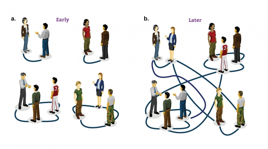
From a Cocktail Party to Random Networks
The emergence of an acquaintance network through random encounters at a cocktail party.
Early on the guests form isolated groups.
As individuals mingle, changing groups, an invisible network emerges that connects all of them into a single network.
Section 3.2
The Random Network Model
Network science aims to build models that reproduce the properties of real networks. Most networks we encounter do not have the comforting regularity of a crystal lattice or the predictable radial architecture of a spider web. Rather, at first inspection they look as if they were spun randomly (Image 2.4). Random network theory embraces this apparent randomness by constructing and characterizing networks that are truly random.
From a modeling perspective a network is a relatively simple object, consisting of only nodes and links. The real challenge, however, is to decide where to place the links between the nodes so that we reproduce the complexity of a real system. In this respect the philosophy behind a random network is simple: We assume that this goal is best achieved by placing the links randomly between the nodes. That takes us to the definition of a random network (BOX 3.1):
A random network consists of N nodes where each node pair is connected with probability p.
To construct a random network we follow these steps:
Start with N isolated nodes.
Select a node pair and generate a random number between 0 and 1. If the number exceeds p, connect the selected node pair with a link, otherwise leave them disconnected.
Repeat step (2) for each of the N(N-1)/2 node pairs.
The network obtained after this procedure is called a random graph or a random network. Two mathematicians, Pál Erdős and Alfréd Rényi, have played an important role in understanding the properties of these networks. In their honor a random network is called the Erdős-Rényi network (BOX 3.2).
Section 3.3
Number of Links
Each random network generated with the same parameters N, p looks slightly different (Image 3.3). Not only the detailed wiring diagram changes between realizations, but so does the number of links L. It is useful, therefore, to determine how many links we expect for a particular realization of a random network with fixed Nand p.
The probability that a random network has exactly L links is the product of three terms:
The probability that L of the attempts to connect the N(N-1)/2 pairs of nodes have resulted in a link, which is pL.
The probability that the remaining N(N-1)/2 - L attempts have not resulted in a link, which is (1-p)N(N-1)/2-L.
A combinational factor,
counting the number of different ways we can place L links among N(N-1)/2 node pairs.
We can therefore write the probability that a particular realization of a random network has exactly L links as
As (3.1) is a binomial distribution (BOX 3.3), the expected number of links in a random graph is
\
Hence ‹L› is the product of the probability p that two nodes are connected and the number of pairs we attempt to connect, which is Lmax = N(N - 1)/2 (CHAPTER 2).
Using (3.2) we obtain the average degree of a random network
Hence ‹k› is the product of the probability p that two nodes are connected and (N-1), which is the maximum number of links a node can have in a network of size N.
In summary the number of links in a random network varies between realizations. Its expected value is determined by N and p. If we increase p a random network becomes denser: The average number of links increase linearly from ‹L› = 0 to Lmax and the average degree of a node increases from ‹k› = 0 to ‹k› = N-1.
Image 3.3
Random Networks are Truly Random
Top Row
Three realizations of a random network generated with the same parameters p=1/6 and N=12. Despite the identical parameters, the networks not only look different, but they have a different number of links as well (L=10, 10, 8).
Bottom Row
Three realizations of a random network with p=0.03 and N=100. Several nodes have degree k=0, shown as isolated nodes at the bottom.
Section 3.4
Degree Distribution
In a given realization of a random network some nodes gain numerous links, while others acquire only a few or no links (Image 3.3). These differences are captured by the degree distribution, pk, which is the probability that a randomly chosen node has degree k. In this section we derive pk for a random network and discuss its properties.
Image 3.4
Binomial vs. Poisson Degree Distribution
The exact form of the degree distribution of a random network is the binomial distribution(left half). For N ›› ‹k› the binomial is well approximated by a Poisson distribution (right half). As both formulas describe the same distribution,they have the identical properties, but they are expressed in terms of different parameters: The binomial distribution depends on p and N, while the Poisson distribution has only one parameter, ‹k›. It is this simplicity that makes the Poisson form preferred in calculations.
Binomial Distribution
In a random network the probability that node i has exactly k links is the product of three terms [15]:
The probability that k of its links are present, or pk.
The probability that the remaining (N-1-k) links are missing, or (1-p)N-1-k
The number of ways we can select k links from N- 1 potential links a node can have, or
Consequently the degree distribution of a random network follows the binomial distribution
The shape of this distribution depends on the system size N and the probability p (Image 3.4). The binomial distribution (BOX 3.3) allows us to calculate the network’s average degree ‹k›, recovering (3.3), as well as its second moment ‹k2› and variance σk (Image 3.4).
Poisson Distribution
Most real networks are sparse, meaning that for them ‹k› ‹‹ N (Table 2.1). In this limit the degree distribution (3.7) is well approximated by the Poisson distribution (ADVANCED TOPICS 3.A)
which is often called, together with (3.7), the degree distribution of a random network.
The binomial and the Poisson distribution describe the same quantity, hence they have similar properties (Image 3.4):
Both distributions have a peak around ‹k›. If we increase p the network becomes denser, increasing ‹k› and moving the peak to the right.
The width of the distribution (dispersion) is also controlled by p or ‹k›. The denser the network, the wider is the distribution, hence the larger are the differences in the degrees.
When we use the Poisson form (3.8), we need to keep in mind that:
The exact result for the degree distribution is the binomial form (3.7), thus (3.8) represents only an approximation to (3.7) valid in the ‹k› ‹‹ N limit. As most networks of practical importance are sparse, this condition is typically satisfied.
The advantage of the Poisson form is that key network characteristics, like <‹k›, ‹k2› and σk , have a much simpler form (Image 3.4), depending on a single parameter, ‹k›.
The Poisson distribution in (3.8) does not explicitly depend on the number of nodes N. Therefore, (3.8) predicts that the degree distribution of networks of different sizes but the same average degree ‹k› are indistinguishable from each other (Image 3.5).
In summary, while the Poisson distribution is only an approximation to the degree distribution of a random network, thanks to its analytical simplicity, it is the preferred form for pk. Hence throughout this book, unless noted otherwise, we will refer to the Poisson form (3.8) as the degree distribution of a random network. Its key feature is that its properties are independent of the network size and depend on a single parameter, the average degree ‹k›.
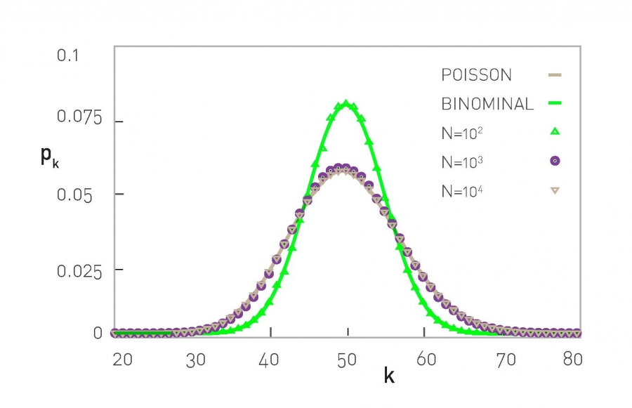
Image 3.5
Degree Distribution is Independent of the Network Size
The degree distribution of a random network with ‹k› = 50 and N = 102, 103, 104.
Small Networks: Binomial
For a small network (N = 102) the degree distribution deviates significantly from the Poisson form (3.8), as the condition for the Poisson approximation, N»‹k›, is not satisfied. Hence for small networks one needs to use the exact binomial form (3.7) (green line).
Large Networks: Poisson
For larger networks (N = 103, 104) the degree distribution becomes indistinguishable from the Poisson prediction (3.8), shown as a continuous grey line. Therefore for large N the degree distribution is independent of the network size. In the figure we averaged over 1,000 independently generated random networks to decrease the noise.
Section 3.5
Real Networks are Not Poisson
As the degree of a node in a random network can vary between 0 and N-1, we must ask, how big are the differences between the node degrees in a particular realization of a random network? That is, can high degree nodes coexist with small degree nodes? We address these questions by estimating the size of the largest and the smallest node in a random network.
Let us assume that the world’s social network is described by the random network model. This random society may not be as far fetched as it first sounds: There is significant randomness in whom we meet and whom we choose to become acquainted with.
Sociologists estimate that a typical person knows about 1,000 individuals on a first name basis, prompting us to assume that ‹k› ≈ 1,000. Using the results obtained so far about random networks, we arrive to a number of intriguing conclusions about a random society of N ≈ 7 x 10⁹ of individuals (ADVANCED TOPICS 3.B):
The most connected individual (the largest degree node) in a random society is expected to have kmax = 1,185 acquaintances.
The degree of the least connected individual is kmin = 816, not that different from kmax or ‹k›.
The dispersion of a random network is σk = ‹k›1/2 , which for ‹k› = 1,000 is σk = 31.62. This means that the number of friends a typical individual has is in the ‹k› ± σk range, or between 968 and 1,032, a rather narrow window.
Taken together, in a random society all individuals are expected to have a comparable number of friends. Hence if people are randomly connected to each other, we lack outliers: There are no highly popular individuals, and no one is left behind, having only a few friends. This suprising conclusion is a consequence of an important property of random networks: in a large random network the degree of most nodes is in the narrow vicinity of ‹k›
This prediction blatantly conflicts with reality. Indeed, there is extensive evidence of individuals who have considerably more than 1,185 acquaintances. For example, US president Franklin Delano Roosevelt’s appointment book has about 22,000 names, individuals he met personally [16, 17]. Similarly, a study of the social network behind Facebook has documented numerous individuals with 5,000 Facebook friends, the maximum allowed by the social networking platform [18]. To understand the origin of these discrepancies we must compare the degree distribution of real and random networks.
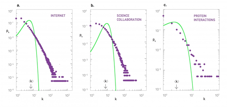
Image 3.6
Degree Distribution of Real Networks
The degree distribution of the (a) Internet, (b) science collaboration network, and (c) protein interaction network (Table 2.1). The green line corresponds to the Poisson prediction, obtained by measuring ‹k› for the real network and then plotting (3.8). The significant deviation between the data and the Poisson fit indicates that the random network model underestimates the size and the frequency of the high degree nodes, as well as the number of low degree nodes. Instead the random network model predicts a larger number of nodes in the vicinity of ‹k› than seen in real networks.
Section 3.6
The Evolution of a Random Network
The cocktail party we encountered at the beginning of this chapter captures a dynamical process: Starting with N isolated nodes, the links are added gradually through random encounters between the guests. This corresponds to a gradual increase of p, with striking consequences on the network topology (Video 3.2). To quantify this process, we first inspect how the size of the largest connected cluster within the network, NG, varies with ‹k›. Two extreme cases are easy to understand:
For p = 0 we have ‹k› = 0, hence all nodes are isolated. Therefore the largest component has size NG = 1 and NG/N→0 for large N.
For p = 1 we have ‹k›= N-1, hence the network is a complete graph and all nodes belong to a single component. Therefore NG = N and NG/N = 1.
Video 3.2 Evolution of a Random Network
A video showing the change in the structure of a random network with increasing p. It vividly illustrates the absence of a giant component for small p and its sudden emergence once p reaches a critical value.
One would expect that the largest component grows gradually from NG = 1 to NG = N if ‹k› increases from 0 to N-1. Yet, as Image 3.7a indicates, this is not the case: NG/N remains zero for small ‹k›, indicating the lack of a large cluster. Once ‹k› exceeds a critical value, NG/N increases, signaling the rapid emergence of a large cluster that we call the giant component. Erdős and Rényi in their classical 1959 paper predicted that the condition for the emergence of the giant component is [2]
In other words, we have a giant component if and only if each node has on average more than one link (ADVANCED TOPICS 3.C).
The fact that we need at least one link per node to observe a giant component is not unexpected. Indeed, for a giant component to exist, each of its nodes must be linked to at least one other node. It is somewhat counterintuitive, however, that one link is sufficient for its emergence.
We can express (3.10) in terms of p using (3.3), obtaining
Therefore the larger a network, the smaller p is sufficient for the giant component.
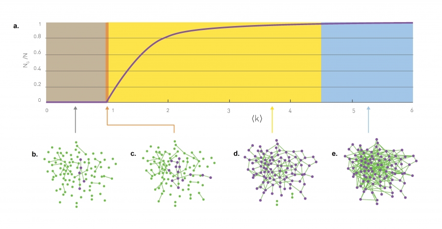
The emergence of the giant component is only one of the transitions characterizing a random network as we change ‹k›. We can distinguish four topologically distinct regimes (Image 3.7a), each with its unique characteristics:
For ‹k› = 0 the network consists of N isolated nodes. Increasing ‹k› means that we are adding N‹k› = pN(N-1)/2 links to the network. Yet, given that ‹k› ‹ 1, we have only a small number of links in this regime, hence we mainly observe tiny clusters (Image 3.7b).
We can designate at any moment the largest cluster to be the giant component. Yet in this regime the relative size of the largest cluster, NG/N, remains zero. The reason is that for ‹k› ‹ 1 the largest cluster is a tree with size NG ~ lnN, hence its size increases much slower than the size of the network. Therefore NG/N ≃ lnN/N→0 in the N→∞ limit.
In summary, in the subcritical regime the network consists of numerous tiny components, whose size follows the exponential distribution (3.35). Hence these components have comparable sizes, lacking a clear winner that we could designate as a giant component.
The critical point separates the regime where there is not yet a giant component (‹k› ‹ 1) from the regime where there is one (‹k› › 1). At this point the relative size of the largest component is still zero (Image 3.7c). Indeed, the size of the largest component is NG ~ N2/3. Consequently NG grows much slower than the network’s size, so its relative size decreases as NG/N ~ N-1/3 in the N→∞ limit.
Note, however, that in absolute terms there is a significant jump in the size of the largest component at ‹k› = 1. For example, for a random network with N = 7 ×10⁹ nodes, comparable to the globe’s social network, for ‹k› ‹ 1 the largest cluster is of the order of NG ≃ lnN = ln (7 ×10⁹) ≃ 22.7. In contrast at ‹k› = 1 we expect NG ~ N2/3 = (7 ×10⁹)2/3 ≃ 3 ×10⁶, a jump of about five orders of magnitude. Yet, both in the subcritical regime and at the critical point the largest component contains only a vanishing fraction of the total number of nodes in the network.
In summary, at the critical point most nodes are located in numerous small components, whose size distribution follows (3.36). The power law form indicates that components of rather different sizes coexist. These numerous small components are mainly trees, while the giant component may contain loops. Note that many properties of the network at the critical point resemble the properties of a physical system undergoing a phase transition (ADVANCED TOPICS 3.F).
Image 3.7
Evolution of a Random Network
The relative size of the giant component in function of the average degree ‹k› in the Erdős-Rényi model. The figure illustrates the phase tranisition at ‹k› = 1, responsible for the emergence of a giant component with nonzero NG
A sample network and its properties in the four regimes that characterize a random network.
This regime has the most relevance to real systems, as for the first time we have a giant component that looks like a network. In the vicinity of the critical point the size of the giant component varies as
or
where pc is given by (3.11). In other words, the giant component contains a finite fraction of the nodes. The further we move from the critical point, a larger fraction of nodes will belong to it. Note that (3.12) is valid only in the vicinity of ‹k› = 1. For large ‹k› the dependence between NG and ‹k› is nonlinear (Image 3.7a).
In summary in the supercritical regime numerous isolated components coexist with the giant component, their size distribution following (3.35). These small components are trees, while the giant component contains loops and cycles. The supercritical regime lasts until all nodes are absorbed by the giant component.
For sufficiently large p the giant component absorbs all nodes and components, hence NG≃ N. In the absence of isolated nodes the network becomes connected. The average degree at which this happens depends on N as (ADVANCED TOPIC 3.E)
Note that when we enter the connected regime the network is still relatively sparse, as lnN / N → 0 for large N. The network turns into a complete graph only at ‹k› = N - 1.
In summary, the random network model predicts that the emergence of a network is not a smooth, gradual process: The isolated nodes and tiny components observed for small ‹k› collapse into a giant component through a phase transition (ADVANCED TOPICS 3.F). As we vary ‹k› we encounter four topologically distinct regimes (Image 3.7).
The discussion offered above follows an empirical perspective, fruitful if we wish to compare a random network to real systems. A different perspective, with its own rich behavior, is offered by the mathematical literature (BOX 3.5).
Section 3.7
Real Networks are Supercritical
Two predictions of random network theory are of direct importance for real networks:
Once the average degree exceeds ‹k› = 1, a giant component should emerge that contains a finite fraction of all nodes. Hence only for ‹k› › 1 the nodes organize themselves into a recognizable network.
For ‹k› › lnN all components are absorbed by the giant component, resulting in a single connected network.
Do real networks satisfy the criteria for the existence of a giant component, i.e. ‹k› › 1? And will this giant component contain all nodes for ‹k› › lnN, or will we continue to see some disconnected nodes and components? To answer these questions we compare the structure of a real network for a given ‹k› with the theoretical predictions discussed above.
The measurements indicate that real networks extravagantly exceed the ‹k› = 1 threshold. Indeed, sociologists estimate that an average person has around 1,000 acquaintances; a typical neuron is the human brain has about 7,000 synapses; in our cells each molecule takes part in several chemical reactions.
This conclusion is supported by Table 3.1, that lists the average degree of several undirected networks, in each case finding ‹k› › 1. Hence the average degree of real networks is well beyond the ‹k› = 1 threshold, implying that they all have a giant component. The same is true for the reference networks listed in Table 3.1.
Network
N
L
‹K›
lnN
Internet
192,244
609,066
6.34
12.17
Power Grid
4,941
6,594
2.67
8.51
Science Collaboration
23,133
94,437
8.08
10.05
Actor Network
702,388
29,397,908
83.71
13.46
Protein Interactions
2,018
2,930
2.90
7.61
Table 3.1
Are Real Networks Connected?
The number of nodes N and links L for the undirected networks of our reference network list of Table 3.1, shown together with ‹k› and lnN. A giant component is expected for ‹k› › 1 and all nodes should join the giant component for ‹k› › lnN. While for all networks ‹k› › 1, for most ‹k› is under the lnN threshold (see also Image 3.9).
Let us now turn to the second prediction, inspecting if we have single component (i.e. if ‹k› › lnN), or if the network is fragmented into multiple components (i.e. if ‹k› ‹ lnN). For social networks the transition between the supercritical and the fully connected regime should be at ‹k› › ln(7×10⁹) ≈ 22.7. That is, if the average individual has more than two dozens acquaintances, then a random society must have a single component, leaving no individual disconnected. With ‹k› ≈ 1,000 this condition is clearly satisfied. Yet, according to Table 3.1 many real networks do not obey the fully connected criteria. Consequently, according to random network theory these networks should be fragmented into several disconnected components. This is a disconcerting prediction for the Internet, indicating that some routers should be disconnected from the giant component, being unable to communicate with other routers. It is equally problematic for the power grid, indicating that some consumers should not get power. These predictions are clearly at odds with reality.
In summary, we find that most real networks are in the supercritical regime (Image 3.9). Therefore these networks are expected to have a giant component, which is in agreement with the observations. Yet, this giant component should coexist with many disconnected components, a prediction that fails for several real networks. Note that these predictions should be valid only if real networks are accurately described by the Erdős-Rényi model, i.e. if real networks are random. In the coming chapters, as we learn more about the structure of real networks, we will understand why real networks can stay connected despite failing the ‹k› › lnNcriteria.
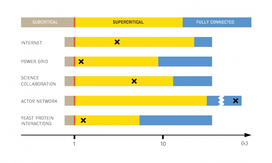
Image 3.9
Most Real Networks are Supercritical
The four regimes predicted by random network theory, marking with a cross the location (‹k›) of the undirected networks listed in Table 3.1. The diagram indicates that most networks are in the supercritical regime, hence they are expected to be broken into numerous isolated components. Only the actor network is in the connected regime, meaning that all nodes are part of a single giant component. Note that while the boundary between the subcritical and the supercritical regime is always at ‹k› = 1, the boundary between the supercritical and the connected regime is at lnN, which varies from system to system.
Section 3.8
Small Worlds
The small world phenomenon, also known as six degrees of separation, has long fascinated the general public. It states that if you choose any two individuals anywhere on Earth, you will find a path of at most six acquaintances between them (Image 3.10). The fact that individuals who live in the same city are only a few handshakes from each other is by no means surprising. The small world concept states, however, that even individuals who are on the opposite side of the globe can be connected to us via a few acquaintances.
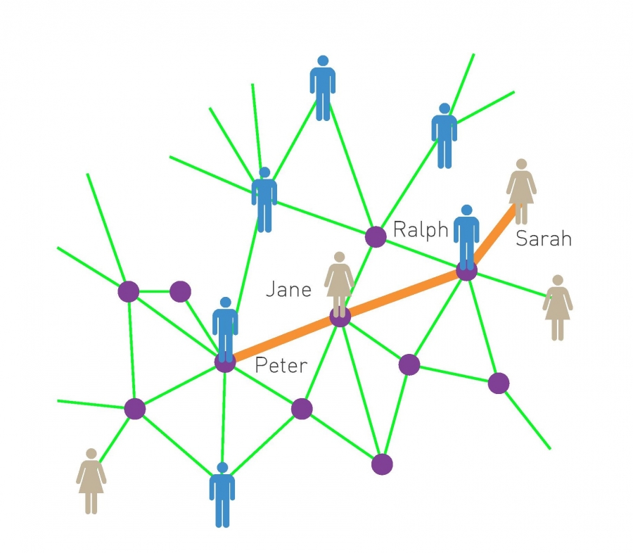
Image 3.10
Six Deegree of Separation
According to six degrees of separation two individuals, anywhere in the world, can be connected through a chain of six or fewer acquaintances. This means that while Sarah does not know Peter, she knows Ralph, who knows Jane and who in turn knows Peter. Hence Sarah is three handshakes, or three degrees from Peter. In the language of network science six degrees, also called the small world property, means that the distance between any two nodes in a network is unexpectedly small.
In the language of network science the small world phenomenon implies that the distance between two randomly chosen nodes in a network is short. This statement raises two questions: What does short (or small) mean, i.e. short compared to what? How do we explain the existence of these short distances?
Both questions are answered by a simple calculation. Consider a random network with average degree ‹k›. A node in this network has on average:
‹k› nodes at distance one (d=1).
‹k›2 nodes at distance two (d=2).
‹k›3 nodes at distance three (d =3).
...
‹k›d nodes at distance d.
For example, if ‹k› ≈ 1,000, which is the estimated number of acquaintences an individual has, we expect 106 individuals at distance two and about a billion, i.e. almost the whole earth’s population, at distance three from us.
To be precise, the expected number of nodes up to distance d from our starting node is
N(d) must not exceed the total number of nodes, N, in the network. Therefore the distances cannot take up arbitrary values. We can identify the maximum distance, dmax, or the network’s diameter by setting
Assuming that ‹k› » 1, we can neglect the (-1) term in the nominator and the denominator of (3.15), obtaining
Therefore the diameter of a random network follows
which represents the mathematical formulation of the small world phenomenon. The key, however is its interpretation:
As derived, (3.18) predicts the scaling of the network diameter, dmax, with the size of the system, N. Yet, for most networks (3.18) offers a better approximation to the average distance between two randomly chosen nodes, ‹d›, than to dmax (Table 3.2). This is because dmax is often dominated by a few extreme paths, while ‹d› is averaged over all node pairs, a process that supresses the fluctuations. Hence typically the small world property is defined by
describing the dependence of the average distance in a network on N and ‹k›.
In general lnN « N, hence the dependence of ‹d› on lnN implies that the distances in a random network are orders of magnitude smaller than the size of the network. Consequently by small in the "small world phenomenon" we mean that the average path length or the diameter depends logarithmically on the system size. Hence, “small” means that ‹d› is proportional to lnN, rather than N or some power of N (Image 3.11).
The 1/ln ‹k› term implies that the denser the network, the smaller is the distance between the nodes.
In real networks there are systematic corrections to (3.19), rooted in the fact that the number of nodes at distance d › ‹d› drops rapidly (ADVANCED TOPICS 3.F).
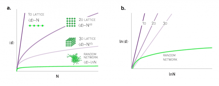
Image 3.11
Why are Small Worlds Surprising?
Much of our intuition about distance is based on our experience with regular lattices, which do not display the small world property:
1D: For a one-dimensional lattice (a line of length N) the diameter and the average path length scale linearly with N: dmax~‹d› ~N.
2D: For a square lattice dmax~‹d› ~ N1/2.
3D: For a cubic lattice dmax~‹d› ~ N1/3.
4D: In general, for a d-dimensional lattice dmax~‹d› ~ N1/d.
These polynomial dependences predict a much faster increase with N than (3.19), indicating that in lattices the path lengths are significantly longer than in a random network. For example, if the social network would form a square lattice (2D), where each individual knows only its neighbors, the average distance between two individuals would be roughly (7 ×10⁹)1/2 = 83,666. Even if we correct for the fact that a person has about 1,000 acquaintances, not four, the average separation will be orders of magnitude larger than predicted by (3.19).
The figure shows the predicted N-dependence of ‹d› for regular and random networks on a linear scale.
The same as in (a), but shown on a log-log scale.
Let us illustrate the implications of (3.19) for social networks. Using N ≈ 7 ×10⁹ and ‹k› ≈ 103, we obtain
Therefore, all individuals on Earth should be within three to four handshakes of each other [20]. The estimate (3.20) is probably closer to the real value than the frequently quoted six degrees (BOX 3.7).
Much of what we know about the small world property in random networks, including the result (3.19), is in a little known paper by Manfred Kochen and Ithiel de Sola Pool [20], in which they mathematically formulated the problem and discussed in depth its sociological implications. This paper inspired the well known Milgram experiment (BOX 3.6), which in turn inspired the six-degrees of separation phrase.
While discovered in the context of social systems, the small world property applies beyond social networks (BOX 3.6). To demonstrate this in Table 3.2 we compare the prediction of (3.19) with the average path length ‹d› for several real networks, finding that despite the diversity of these systems and the significant differences between them in terms of N and ‹k›, (3.19) offers a good approximation to the empirically observed ‹d›.
In summary the small world property has not only ignited the public’s imagination (BOX 3.8), but plays an important role in network science as well. The small world phenomena can be reasonably well understood in the context of the random network model: It is rooted in the fact that the number of nodes at distance d from a node increases exponentially with d. In the coming chapters we will see that in real networks we encounter systematic deviations from (3.19), forcing us to replace it with more accurate predictions. Yet the intuition offered by the random network model on the origin of the small world phenomenon remains valid.
Network
N
L
‹k›
‹d›
dmax
lnN/ln‹k›
Internet
192,244
609,066
6.34
6.98
26
6.58
WWW
325,729
1,497,134
4.60
11.27
93
8.31
Power Grid
4,941
6,594
2.67
18.99
46
8.66
Mobile-Phone Calls
36,595
91,826
2.51
11.72
39
11.42
Email
57,194
103,731
1.81
5.88
18
18.4
Science Collaboration
23,133
93,437
8.08
5.35
15
4.81
Actor Network
702,388
29,397,908
83.71
3.91
14
3.04
Citation Network
449,673
4,707,958
10.43
11.21
42
5.55
E. Coli Metabolism
1,039
5,802
5.58
2.98
8
4.04
Protein Interactions
2,018
2,930
2.90
5.61
14
7.14
Table 3.2
Six Degrees of Separation
The average distance ‹d› and the maximum distance dmax for the ten reference networks. The last column provides ‹d› predicted by (3.19), indicating that it offers a reasonable approximation to the measured ‹d›. Yet, the agreement is not perfect - we will see in the next chapter that for many real networks (3.19) needs to be adjusted. For directed networks the average degree and the path lengths are measured along the direction of the links.
Section 3.9
Clustering Coefficient
The degree of a node contains no information about the relationship between a node's neighbors. Do they all know each other, or are they perhaps isolated from each other? The answer is provided by the local clustering coefficient Ci, that measures the density of links in node i’s immediate neighborhood: Ci = 0 means that there are no links between i’s neighbors; Ci = 1 implies that each of the i’s neighbors link to each other (SECTION 2.10).
To calculate Ci for a node in a random network we need to estimate the expected number of links Li between the node’s ki neighbors. In a random network the probability that two of i’s neighbors link to each other is p. As there are ki(ki - 1)/2 possible links between the ki neighbors of node i, the expected value of Li is
Thus the local clustering coefficient of a random network is
Equation (3.21) makes two predictions:
For fixed ‹k›, the larger the network, the smaller is a node’s clustering coefficient. Consequently a node's local clustering coefficient Ci is expected to decrease as 1/N. Note that the network's average clustering coefficient, ‹C› also follows (3.21).
The local clustering coefficient of a node is independent of the node’s degree.
To test the validity of (3.21) we plot ‹C›/‹k› in function of N for several undirected networks (Image 3.13a). We find that ‹C›/‹k› does not decrease as N-1, but it is largely independent of N, in violation of the prediction (3.21) and point (1) above. In Image 3.13b-d we also show the dependency of C on the node’s degree ki for three real networks, finding that C(k) systematically decreases with the degree, again in violation of (3.21) and point (2).
In summary, we find that the random network model does not capture the clustering of real networks. Instead real networks have a much higher clustering coefficient than expected for a random network of similar N and L. An extension of the random network model proposed by Watts and Strogatz [29] addresses the coexistence of high ‹C› and the small world property (BOX 3.9). It fails to explain, however, why high-degree nodes have a smaller clustering coefficient than low-degree nodes. Models explaining the shape of C(k) are discussed in Chapter 9.
Image 3.13
Clustering in Real Networks
Comparing the average clustering coefficient of real networks with the prediction (3.21) for random networks. The circles and their colors correspond to the networks of Table 3.2. Directed networks were made undirected to calculate ‹C› and ‹k›. The green line corresponds to (3.21), predicting that for random networks the average clustering coefficient decreases as N-1. In contrast, for real networks ‹C› appears to be independent of N.
The dependence of the local clustering coefficient, C(k), on the node’s degree for (b) the Internet, (c) science collaboration network and (d) protein interaction network. C(k) is measured by averaging the local clustering coefficient of all nodes with the same degree k. The green horizontal line corresponds to ‹C›.
Section 3.10
Summary: Real Networks are Not Random
Since its introduction in 1959 the random network model has dominated mathematical approaches to complex networks. The model suggests that the random-looking networks observed in complex systems should be described as purely random. With that it equated complexity with randomness. We must therefore ask:
Do we really believe that real networks are random?
The answer is clearly no. As the interactions between our proteins are governed by the strict laws of biochemistry, for the cell to function its chemical architecture cannot be random. Similarly, in a random society an American student would be as likely to have among his friends Chinese factory workers than one of her classmates.
In reality we suspect the existence of a deep order behind most complex systems. That order must be reflected in the structure of the network that describes their architecture, resulting in systematic deviations from a pure random configuration.
The degree to which random networks describe, or fail to describe, real systems, must not be decided by epistemological arguments, but by a systematic quantitative comparison. We can do this, taking advantage of the fact that random network theory makes a number of quantitative predictions:
Degree Distribution
A random network has a binomial distribution, well approximated by a Poisson distribution in the k « N limit. Yet, as shown in Image 3.5, the Poisson distribution fails to capture the degree distribution of real networks. In real systems we have more highly connected nodes than the random network model could account for.
Connectedness
Random network theory predicts that for ‹k› › 1 we should observe a giant component, a condition satisfied by all networks we examined. Most networks, however, do not satisfy the ‹k› › lnN condition, implying that they should be broken into isolated clusters (Table 3.1). Some networks are indeed fragmented, most are not.
Average Path Length
Random network theory predicts that the average path length follows (3.19), a prediction that offers a reasonable approximation for the observed path lengths. Hence the random network model can account for the emergence of small world phenomena.
Clustering Coefficient
In a random network the local clustering coefficient is independent of the node’s degree and ‹C› depends on the system size as 1/N. In contrast, measurements indicate that for real networks C(k) decreases with the node degrees and is largely independent of the system size (Image 3.13).
Taken together, it appears that the small world phenomena is the only property reasonably explained by the random network model. All other network characteristics, from the degree distribution to the clustering coefficient, are significantly different in real networks. The extension of the Erdős-Rényi model proposed by Watts and Strogatz successfully predicts the coexistence of high C and low ‹d›, but fails to explain the degree distribution and C(k). In fact, the more we learn about real networks, the more we will arrive at the startling conclusion that we do not know of any real network that is accurately described by the random network model.
This conclusion begs a legitimate question: If real networks are not random, why did we devote a full chapter to the random network model? The answer is simple: The model serves as an important reference as we proceed to explore the properties of real networks. Each time we observe some network property we will have to ask if it could have emerged by chance. For this we turn to the random network model as a guide: If the property is present in the model, it means that randomness can account for it. If the property is absent in random networks, it may represent some signature of order, requiring a deeper explanation. So, the random network model may be the wrong model for most real systems, but it remains quite relevant for network science (BOX 3.10).
Section 3.11
Homework
Erdős-Rényi Networks
Consider an Erdős-Rényi network with N = 3,000 nodes, connected to each other with probability p = 10–3.
What is the expected number of links, 〈L〉?
In which regime is the network?
Calculate the probability pc so that the network is at the critical point
Given the linking probability p = 10–3, calculate the number of nodes Ncr so that the network has only one component.
For the network in (d), calculate the average degree 〈kcr〉 and the average distance between two randomly chosen nodes 〈d〉.
Calculate the degree distribution pk of this network (approximate with a Poisson degree distribution).
Generating Erdős-Rényi Networks
Relying on the G(N, p) model, generate with a computer three networks with N = 500 nodes and average degree (a) 〈k〉 = 0.8, (b) 〈k〉 = 1 and (c) 〈k〉 = 8. Visualize these networks.
Circle Network
Consider a network with N nodes placed on a circle, so that each node connects to m neighbors on either side (consequently each node has degree 2m). Image 3.14(a) shows an example of such a network with m = 2 and N = 20. Calculate the average clustering coefficient 〈C〉 of this network and the average shortest path 〈d〉. For simplicity assume that N and m are chosen such that (n-1)/2m is an integer. What happens to 〈C〉 if N≫1? And what happens to 〈d〉?
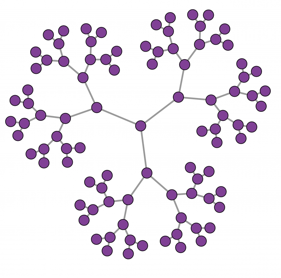
Cayley Tree
A Cayley tree is a symmetric tree, constructed starting from a central node of degree k. Each node at distance d from the central node has degree k, until we reach the nodes at distance P that have degree one and are called leaves (see Image 3.16 for a Cayley tree with k = 3 and P = 5.)
Calculate the number of nodes reachable in t steps from the central node.
Calculate the degree distribution of the network.
Calculate the diameter dmax.
Find an expression for the diameter dmax in terms of the total number of nodes N.
Does the network display the small-world property?
Snobbish Network
Consider a network of N red and N blue nodes. The probability that there is a link between nodes of identical color is p and the probability that there is a link between nodes of different color is q. A network is snobbish if p › q, capturing a tendency to connect to nodes of the same color. For q = 0 the network has at least two components, containing nodes with the same color.
Calculate the average degree of the "blue" subnetwork made of only blue nodes, and the average degree in the full network.
Determine the minimal p and q required to have, with high probability, just one component.
Show that for large N even very snobbish networks (p≫q) display the small-world property.
Snobbish Social Networks
Consider the following variant of the model discussed above: We have a network of 2N nodes, consisting of an equal number of red and blue nodes, while an f fraction of the 2N nodes are purple. Blue and red nodes do not connect to each other (q = 0), while they connect with probability p to nodes of the same color. Purple nodes connect with the same probability p to both red and blue nodes
We call the red and blue communities interactive if a typical red node is just two steps away from a blue node and vice versa. Evaluate the fraction of purple nodes required for the communities to be interactive.
Comment on the size of the purple community if the average degree of the blue (or red) nodes is 〈k〉≫1.
What are the implications of this model for the structure of social (and other) networks?
Image 3.16
Cayley Tree
A Cayley Tree With k = 3 and P = 5.
Section 3.12
Advanced Topic 3.A Deriving the Poisson Distribution
To derive the Poisson form of the degree distribution we start from the exact binomial distribution (3.7)
that characterizes a random graph. We rewrite the first term on the r.h.s. as
where in the last term we used that k « N. The last term of (3.22) can be simplified as
and using the series expansion
we obtain
which is valid if N » k. This represents the small degree approximation at the heart of this derivation. Therefore the last term of (3.22) becomes
Combining (3.22), (3.23), and (3.24) we obtain the Poisson form of the degree distribution
or
Section 3.13
Advanced Topic 3.B Maximum and Minimum Degrees
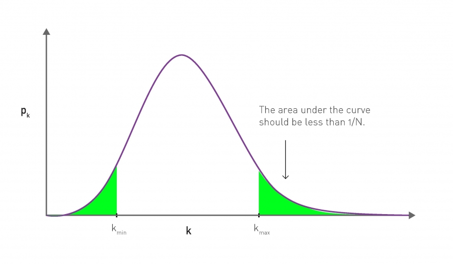
To determine the expected degree of the largest node in a random network, called the network’s upper natural cutoff, we define the degree kmax such that in a network of N nodes we have at most one node with degree higher than kmax . Mathematically this means that the area behind the Poisson distribution pk for k ≥ kmax should be approximately one (Image 3.17). Since the area is given by 1-P(kmax), where P(k) is the cumulative degree distribution of pk, the network’s largest node satisfies:
We write ≈ instead of =, because kmax is an integer, so in general the exact equation does not have a solution. For a Poisson distribution
where in the last term we approximate the sum with its largest term.
For N = 109 and 〈k〉 = 1,000, roughly the size and the average degree of the globe’s social network, (3.26) and (3.27) predict kmax = 1,185, indicating that a random network lacks extremely popular individuals, or hubs.
We can use a similar argument to calculate the expected degree of the smallest node, kmin. By requiring that there should be at most one node with degree smaller than kmin we can write
For the Erdős-Rényi network we have
Solving (3.28) with N = 109 and 〈k〉 = 1,000 we obtain kmin = 816.
Image 3.17
Minimum and Maximum Degree
The estimated maximum degree of a network, kmax, is chosen so that there is at most one node whose degree is higher than kmax. This is often called the natural upper cutoff of a degree distribution. To calculate it, we need to set kmax such that the area under the degree distribution pk for k > kmax equals 1/N, hence the total number of nodes expected in this region is exactly one. We follow a similar argument to determine the expected smallest degree, kmin.
Section 3.14
Advanced Topic 3.C Giant Component
In this section we introduce the argument, proposed independently by Solomonoff and Rapoport [11], and by Erdős and Rényi [2], for the emergence of giant component at 〈k〉= 1 [33].
Let us denote with u = 1 - NG/N the fraction of nodes that are not in the giant component (GC), whose size we take to be NG. If node i is part of the GC, it must link to another node j, which must also be part of the GC. Hence if i is not part of the GC, that could happen for two reasons:
There is no link between i and j (probability for this is 1- p).
There is a link between i and j, but j is not part of the GC (probability for this is pu).
Therefore the total probability that i is not part of the GC via node j is 1 - p + pu. The probability that i is not linked to the GC via any other node is therefore (1 - p + pu)N - 1, as there are N - 1 nodes that could serve as potential links to the GC for node i. As u is the fraction of nodes that do not belong to the GC, for any p and N the solution of the equation
provides the size of the giant component via NG = N(1 - u). Using p = 〈k〉/(N - 1) and taking the logarithm of both sides, for 〈k〉 « N we obtain
where we used the series expansion for ln(1+x).
Taking an exponential of both sides leads to u = exp[- 〈k〉(1 - u)]. If we denote with S the fraction of nodes in the giant component, S = NG / N, then S = 1 - u and (3.31) results in
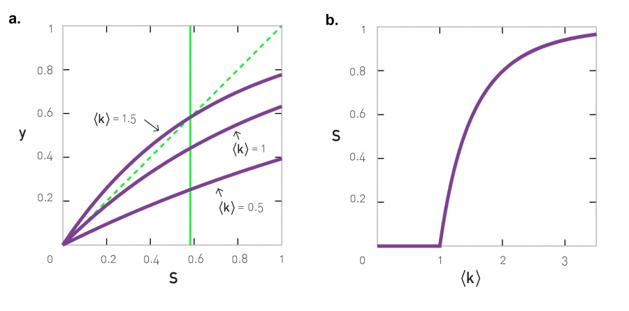
This equation provides the size of the giant component S in function of 〈k〉 (Image 3.18). While (3.32) looks simple, it does not have a closed solution. We can solve it graphically by plotting the right hand side of (3.32) as a function of S for various values of 〈k〉. To have a nonzero solution, the obtained curve must intersect with the dotted diagonal, representing the left hand side of (3.32). For small 〈k〉 the two curves intersect each other only at S = 0, indicating that for small 〈k〉 the size of the giant component is zero. Only when 〈k〉 exceeds a threshold value, does a non-zero solution emerge.
To determine the value of 〈k〉 at which we start having a nonzero solution we take a derivative of (3.32), as the phase transition point is when the r.h.s. of (3.32) has the same derivative as the l.h.s. of (3.32), i.e. when
Setting S = 0, we obtain that the phase transition point is at 〈k〉 = 1 (see also ADVANCED TOPICS 3.F).
Image 3.18
Graphical Solution
The three purple curves correspond to y = 1-exp[ -‹k›S ] for ‹k›=0.5, 1, 1.5. The green dashed diagonal corresponds y = S, and the intersection of the dashed and purple curves provides the solution to (3.32). For ‹k›=0.5 there is only one intersection at S = 0, indicating the absence of a giant component. The ‹k›=1.5 curve has a solution at S = 0.583 (green vertical line). The ‹k›=1 curve is precisely at the critical point, representing the separation between the regime where a nonzero solution for S exists and the regime where there is only the solution at S = 0.
The size of the giant component in function of ‹k› as predicted by (3.32). After [33].
Section 3.15
Advanced Topic 3.D Component Sizes
In Image 3.7 we explored the size of the giant component, leaving an important question open: How many components do we expect for a given ‹k›? What is their size distribution? The aim of this section is to discuss these topics.
Component Size Distribution
For a random network the probability that a randomly chosen node belongs to a component of size s (which is different from the giant component G) is [33]
Replacing ‹k›s-1 with exp[(s-1) ln‹k›] and using the Stirling-formula
for large s we obtain
Therefore the component size distribution has two contributions: a slowly decreasing power law term s-3/2 and a rapidly decreasing exponential term e-(‹k›-1)s+(s-1)ln‹k›. Given that the exponential term dominates for large s, (3.35) predicts that large components are prohibited. At the critical point, ‹k› = 1, all terms in the exponential cancel, hence ps follows the power law
As a power law decreases relatively slowly, at the critical point we expect to observe clusters of widely different sizes, a property consistent with the behavior of a system during a phase transition (ADVANCED TOPICS 3.F). These predictions are supported by the numerical simulations shown in Image 3.19.
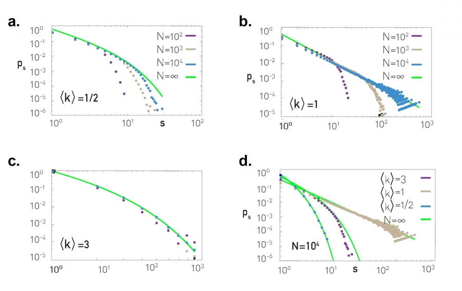
Image 3.19
Component Size Distribution
Component size distribution ps in a random network, excluding the giant component.
ps for different ‹k› values and N, indicating that ps converges for large N to the prediction (3.34).
ps for N = 104, shown for different ‹k›. While for ‹k› ‹ 1 and ‹k› › 1 the ps distribution has an exponential form, right at the critical point ‹k› = 1 the distribution follows the power law (3.36). The continuous green lines correspond to (3.35). The first numerical study of the component size distribution in random networks was carried out in 1998 [34], preceding the exploding interest in complex networks.
Average Component Size
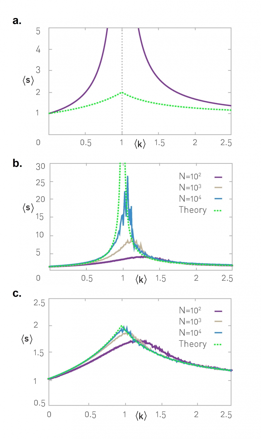
The calculations also indicate that the average component size (once again, excluding the giant component) follows [33]
For ‹k› ‹ 1 we lack a giant component (NG = 0), hence (3.37) becomes
which diverges when the average degree approaches the critical point ‹k› = 1. Therefore as we approach the critical point, the size of the clusters increases, signaling the emergence of the giant component at ‹k› = 1. Numerical simulations support these predictions for large N (Image 3.20).
To determine the average component size for ‹k› › 1 using (3.37), we need to first calculate the size of the giant component. This can be done in a self-consistent manner, obtaining that the average cluster size decreases for ‹k› › 1, as most clusters are gradually absorbed by the giant component.
Note that (3.37) predicts the size of the component to which a randomly chosen node belongs. This is a biased measure, as the chance of belonging to a larger cluster is higher than the chance of belonging to a smaller one. The bias is linear in the cluster size s. If we correct for this bias, we obtain the average size of the small components that we would get if we were to inspect each cluster one by one and then measure their average size [33]
The average size ‹s› of a component to which a randomly chosen node belongs to as predicted by (3.39) (purple). The green curve shows the overall average size ‹s'› of a component as predicted by (3.37). (After [33]).
The average cluster size in a random network. We choose a node and determined the size of the cluster it belongs to. This measure is biased, as each component of size s will be counted s times. The larger N becomes, the more closely the numerical data follows the prediction (3.37). As predicted, ‹s› diverges at the ‹k›=1 critical point, supporting the existence of a phase transition (ADVANCED TOPICS 3.F).
The average cluster size in a random network, where we corrected for the bias in (b) by selecting each component only once.The larger N becomes, the more closely the numerical data follows the prediction (3.39).
To determine the value of ‹k› at which most nodes became part of the giant component, we calculate the probability that a randomly selected node does not have a link to the giant component, which is (1-p)NG≈(1-p)N , as in this regime NG ≃ N. The expected number of such isolated nodes is
where we used (1-x/n)n≈e-x, an approximation valid for large n. If we make p sufficiently large, we arrive to the point where only one node is disconnected from the giant component. At this point IN = 1, hence according to (3.40) p needs to satisfy Ne-Np=1 . Consequently, the value of p at which we are about to enter the fully connected regime is
which leads to (3.14) in terms of ‹k›.
Section 3.17
Advanced Topic 3.F Phase Transitions
The emergence of the giant component at ‹k›=1 in the random network model is reminiscent of a phase transition, a much studied phenomenon in physics and chemistry [35]. Consider two examples:
Water-Ice Transition (Image 3.21a): At high temperatures the H2O molecules engage in a diffusive motion, forming small groups and then breaking apart to group up with other water molecules. If cooled, at 0˚C the molecules suddenly stop this diffusive dance, forming an ordered rigid ice crystal.
Magnetism (Image 3.21b): In ferromagnetic metals like iron at high temperatures the spins point in randomly chosen directions. Under some critical temperature Tc all atoms orient their spins in the same direction and the metal turns into a magnet.
The freezing of a liquid and the emergence of magnetization are examples of phase transitions, representing transitions from disorder to order. Indeed, relative to the perfect order of the crystalline ice, liquid water is rather disordered. Similarly, the randomly oriented spins in a ferromagnet take up the highly ordered common orientation under Tc.
Many properties of a system undergoing a phase transition are universal. This means that the same quantitative patterns are observed in a wide range of systems, from magma freezing into rock to a ceramic material turning into a superconductor. Furthermore, near the phase transition point, called the critical point, many quantities of interest follow power-laws.
The phenomena observed near the critical point ‹k› = 1 in a random network in many ways is similar to a phase transition:
The similarity between Image 3.7a and the magnetization diagram of Image 3.21b is not accidental: they both show a transition from disorder to order. In random networks this corresponds to the emergence of a giant component when ‹k› exceeds ‹k› = 1.
As we approach the freezing point, ice crystals of widely different sizes are observed, and so are domains of atoms with spins pointing in the same direction. The size distribution of the ice crystals or magnetic domains follows a power law. Similarly, while for ‹k› ‹ 1 and ‹k› › 1 the cluster sizes follow an exponential distribution, right at the phase transition point ps follows the power law (3.36), indicating the coexistence of components of widely different sizes.
At the critical point the average size of the ice crystals or of the magnetic domains diverges, assuring that the whole system turns into a single frozen ice crystal or that all spins point in the same direction. Similarly in a random network the average cluster size ‹s› diverges as we approach ‹k› = 1 (Image 3.20).
Image 3.21
Phase Transitions
Water-Ice Phase Transition
The hydrogen bonds that hold the water molecules together (dotted lines) are weak, constantly breaking up and re-forming, maintaining partially ordered local structures (left panel). The temperature-pressure phase diagram indicates (center panel) that by lowering the temperature, the water undergoes a phase transition, moving from a liquid (purple) to a frozen solid (green) phase. In the solid phase each water molecule binds rigidly to four other molecules, forming an ice lattice (right panel). After http://www.lbl.gov/Science-Articles/ Archive/sabl/2005/February/ water-solid.html.
Magnetic Phase Transition
In ferromagnetic materials the magnetic moments of the individual atoms (spins) can point in two different directions. At high temperatures they choose randomly their direction (right panel). In this disordered state the system’s total magnetization (m = ΔM/N, where ΔM is the number of up spins minus the number of down spins) is zero. The phase diagram (middle panel) indicates that by lowering the temperature T, the system undergoes a phase transition at T= Tc, when a nonzero magnetization emerges. Lowering T further allows m to converge to one. In this ordered phase all spins point in the same direction (left panel).
Section 3.18
Advanced Topic 3.G Small World Corrections
Equation (3.18) offers only an approximation to the network diameter, valid for very large N and small d. Indeed, as soon as ‹k›d approaches the system size N the ‹k›d scaling must break down, as we do not have enough nodes to continue the ‹k›d expansion. Such finite size effects result in corrections to (3.18). For a random network with average degree ‹k›, the network diameter is better approximated by [36]
where the Lambert W-function W(z) is the principal inverse of f(z) = z exp(z). The first term on the r.h.s is (3.18), while the second is the correction that depends on the average degree. The correction increases the diameter, accounting for the fact that when we approach the network’s diameter the number of nodes must grow slower than ‹k›. The magnitude of the correction becomes more obvious if we consider the various limits of (3.42).
In the ‹k› → 1 limit we can calculate the Lambert W-function, finding for the diameter [36]
Hence in the moment when the giant component emerges the network diameter is three times our prediction (3.18). This is due to the fact that at the critical point ‹k› = 1 the network has a tree-like structure, consisting of long chains with hardly any loops, a configuration that increases dmax.
In the ‹k› → ∞ limit, corresponding to a very dense network, (3.42) becomes
Hence if ‹k› increases, the second and the third terms vanish and the solution (3.42) converges to the result (3.18).
Section 3.14
Bibliography
[1] A.-L. Barabási. Linked: The new science of networks. Plume Books, 2003.
[2] P. Erdős and A. Rényi. On random graphs, I. Publicationes Mathematicae (Debrecen), 6:290-297, 1959.
[3] P. Erdős and A. Rényi. On the evolution of random graphs. Publ. Math. Inst. Hung. Acad. Sci., 5:17-61, 1960.
[4] P. Erdős and A. Rényi. On the evolution of random graphs. Bull. Inst. Internat. Statist., 38:343-347, 1961.
[5] P. Erdős and A. Rényi. On the Strength of Connectedness of a Random Graph, Acta Math. Acad. Sci. Hungary, 12: 261–267, 1961.
[6] P. Erdős and A. Rényi. Asymmetric graphs. Acta Mathematica Acad. Sci. Hungarica, 14:295-315, 1963.
[7] P. Erdős and A. Rényi. On random matrices. Publ. Math. Inst. Hung. Acad. Sci., 8:455-461, 1966.
[8] P. Erdős and A. Rényi. On the existence of a factor of degree one of a connected random graph. Acta Math. Acad. Sci. Hungary, 17:359-368, 1966.
[9] P. Erdős and A. Rényi. On random matrices II. Studia Sci. Math. Hungary, 13:459-464, 1968.
[10] E. N. Gilbert. Random graphs. The Annals of Mathematical Statistics, 30:1141-1144, 1959.
[11] R. Solomonoff and A. Rapoport. Connectivity of random nets. Bulletin of Mathematical Biology, 13:107-117, 1951.
[12] P. Hoffman. The Man Who Loved Only Numbers: The Story of Paul Erdős and the Search for Mathematical Truth. Hyperion Books, 1998.
[13] B. Schechter. My Brain is Open: The Mathematical Journeys of Paul Erdős. Simon and Schuster, 1998.
[14] G. P. Csicsery. N is a Number: A Portait of Paul Erdős, 1993
[15] B. Bollobás. Random Graphs. Cambridge University Press, 2001.
[16] L. C. Freeman and C. R. Thompson. Estimating Acquaintanceship. Volume, pg. 147-158, in The Small World, Edited by Manfred Kochen (Ablex, Norwood, NJ), 1989.
[17] H. Rosenthal. Acquaintances and contacts of Franklin Roosevelt. Unpublished thesis. Massachusetts Institute of Technology, 1960.
[18] L. Backstrom, P. Boldi, M. Rosa, J. Ugander, and S. Vigna. Four degrees of separation. In ACM Web Science 2012: Conference Proceedings, pages 45−54. ACM Press, 2012.
[19] R. Albert and A.-L. Barabási. Statistical mechanics of complex networks. Reviews of Modern Physics, 74:47-97, 2002.
[20] I. de Sola Pool and M. Kochen. Contacts and Influence. Social Networks, 1: 5-51, 1978.
[21] H. Jeong, R. Albert and A. L. Barabási. Internet: Diameter of the world-wide web. Nature, 401:130-131, 1999.
[22] S. Lawrence and C.L. Giles. Accessibility of information on the Web Nature, 400:107, 1999.
[23] A. Broder, R. Kumar, F. Maghoul, P. Raghavan, S. Rajagopalan, R. Stata, A. Tomkins, and J. Wiener. Graph structure in the web. Computer Networks, 33:309–320, 2000.
[24] S. Milgram. The Small World Problem. Psychology Today, 2: 60-67, 1967.
[25] J. Travers and S. Milgram. An Experimental Study of the Small World Problem. Sociometry, 32:425-443, 1969.
[26] K. Frigyes, “Láncszemek,” in Minden másképpen van (Budapest: Atheneum Irodai es Nyomdai R.-T. Kiadása, 1929), 85–90. English translation is available in [27].
[27] M. Newman, A.-L. Barabási, and D. J. Watts. The Structure and Dynamics of Networks. Princeton University Press, 2006.
[28] J. Guare. Six degrees of separation. Dramatist Play Service, 1992.
[29] D. J. Watts and S. H. Strogatz. Collective dynamics of ‘small-world’ networks. Nature, 393: 409–10, 1998.
[30] T. S. Kuhn. The Structure of Scientific Revolutions. University of Chicago Press, 1962.
[31] A.-L. Barabási and R. Albert. Emergence of scaling in random networks. Science, 286:509-512, 1999.
[32] A.-L. Barabási, R. Albert, and H. Jeong. Meanfield theory for scalefree random networks. Physica A, 272:173-187, 1999.
[33] M. Newman. Networks: An Introduction. Oxford University Press, 2010.
[34] K. Christensen, R. Donangelo, B. Koiller, and K. Sneppen. Evolution of Random Networks. Physical Review Letters, 81:2380-2383, 1998.
[35] H. E. Stanley. Introduction to Phase Transitions and Critical Phenomena. Oxford University Press, 1987.
[36] D. Fernholz and V. Ramachandran. The diameter of sparse random graphs. Random Structures and Algorithms, 31:482-516, 2007.