Hubs represent the most striking difference between a random and a scale-free network. On the World Wide Web, they are websites with an exceptional number of links, like google.com or facebook.com; in the metabolic network they are molecules like ATP or ADP, energy carriers involved in an exceptional number of chemical reactions. The very existence of these hubs and the related scale-free topology raises two fundamental questions:
Why do so different systems as the WWW or the cell converge to a similar scale-free architecture?
Why does the random network model of Erdős and Rényi fail to reproduce the hubs and the power laws observed in real networks?
The first question is particularly puzzling given the fundamental differences in the nature, origin, and scope of the systems that display the scale-free property:
The nodes of the cellular network are metabolites or proteins, while the nodes of the WWW are documents, representing information without a physical manifestation.
The links within the cell are chemical reactions and binding interactions, while the links of the WWW are URLs, or small segments of computer code.
The history of these two systems could not be more different: The cellular network is shaped by 4 billion years of evolution, while the WWW is less than three decades old.
The purpose of the metabolic network is to produce the chemical components the cell needs to stay alive, while the purpose of the WWW is information access and delivery.
To understand why so different systems converge to a similar architecture we need to first understand the mechanism responsible for the emergence of the scale-free property. This is the main topic of this chapter. Given the diversity of the systems that display the scale-free property, the explanation must be simple and fundamental. The answers will change the way we model networks, forcing us to move from describing a network’s topology to modeling the evolution of a complex system.
Video 5.1 Scale-free Sonata
Listen to a recording of Michael Edward Edgerton's 1 sonata for piano, music inspired by scale-free networks.
Section 5.2
Growth and Preferential Attachment
We start our journey by asking: Why are hubs and power laws absent in random networks? The answer emerged in 1999, highlighting two hidden assumptions of the Erdős-Rényi model, that are violated in real networks [1]. Next we discuss these assumptions separately.
Networks Expand Through the Addition of New Nodes
The random network model assumes that we have a fixed number of nodes, N. Yet, in real networks the number of nodes continually grows thanks to the addition of new nodes.
Consider a few examples:
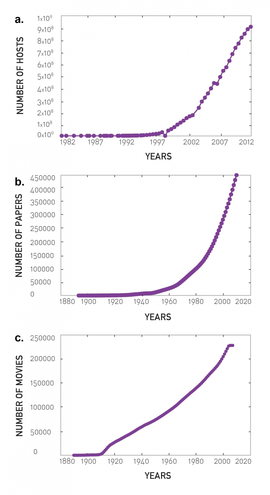
In 1991 the WWW had a single node, the first webpage build by Tim Berners-Lee, the creator of the Web. Today the Web has over a trillion (1012) documents, an extraordinary number that was reached through the continuous addition of new documents by millions of individuals and institutions (Image 5.1a).
The collaboration and the citation network continually expands through the publication of new research papers (Image 5.1b).
The actor network continues to expand through the release of new movies (Image 5.1c).
The protein interaction network may appear to be static, as we inherit our genes (and hence our proteins) from our parents. Yet, it is not: The number of genes grew from a few to the over 20,000 genes present in a human cell over four billion years.
Consequently, if we wish to model these networks, we cannot resort to a static model. Our modeling approach must instead acknowledge that networks are the product of a steady growth process.
Image 5.1
The Growth of Networks
Networks are not static, but grow via the addition of new nodes:
The evolution of the number of WWW hosts, documenting the Web’s rapid growth. After http://www.isc.org/solutions/ survey/history.
The number of scientific papers published in Physical Review since the journal’s founding. The increasing number of papers drives the growth of both the science collaboration network as well as of the citation network shown in the figure.
Number of movies listed in IMDB.com, driving the growth of the actor network.
Nodes Prefer to Link to the More Connected Nodes
The random network model assumes that we randomly choose the interaction partners of a node. Yet, most real networks new nodes prefer to link to the more connected nodes, a process called preferential attachment (Image 5.2).
Consider a few examples:
We are familiar with only a tiny fraction of the trillion or more documents available on the WWW. The nodes we know are not entirely random: We all heard about Google and Facebook, but we rarely encounter the billions of less-prominent nodes that populate the Web. As our knowledge is biased towards the more popular Web documents, we are more likely to link to a high-degree node than to a node with only few links.
No scientist can attempt to read the more than a million scientific papers published each year. Yet, the more cited is a paper, the more likely that we hear about it and eventually read it. As we cite what we read, our citations are biased towards the more cited publications, representing the high-degree nodes of the citation network.
The more movies an actor has played in, the more familiar is a casting director with her skills. Hence, the higher the degree of an actor in the actor network, the higher are the chances that she will be considered for a new role.
In summary, the random network model differs from real networks in two important characteristics:
Growth
Real networks are the result of a growth process that continuously increases N. In contrast the random network model assumes that the number of nodes, N, is fixed.
Preferential Attachment
In real networks new nodes tend to link to the more connected nodes. In contrast nodes in random networks randomly choose their interaction partners.
There are many other differences between real and random networks, some of which will be discussed in the coming chapters. Yet, as we show next, these two, growth and preferential attachment, play a particularly important role in shaping a network’s degree distribution.
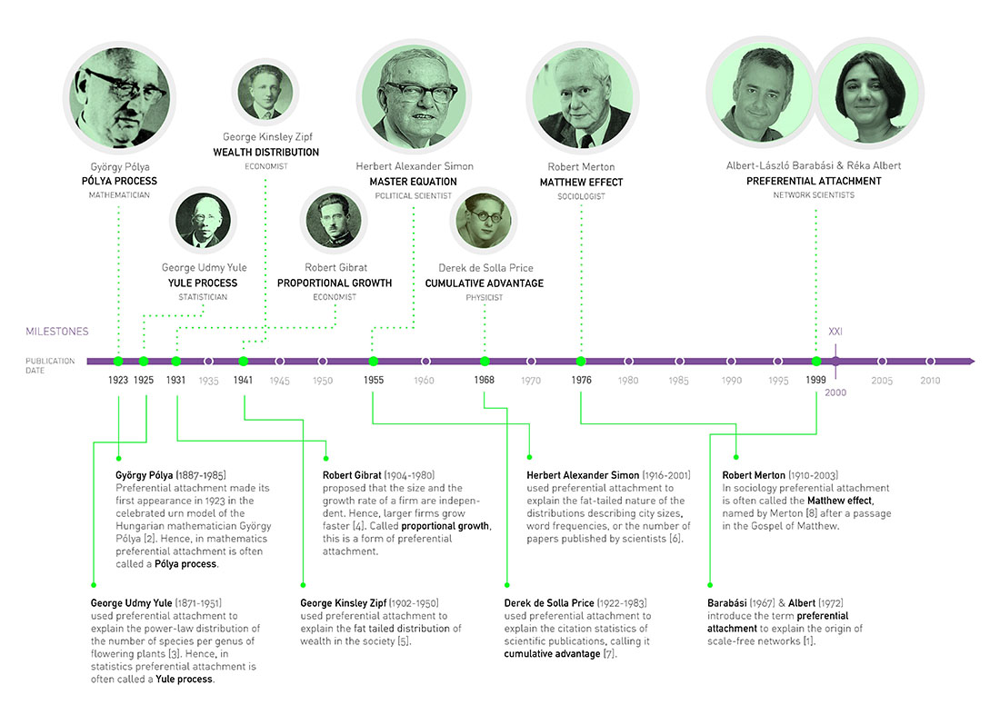
Image 5.2
Preferential Attachment: a Brief History
Section 5.3
The Barabási-Albert Model
The recognition that growth and preferential attachment coexist in real networks has inspired a minimal model called the Barabási-Albert model, which can generate scale-free networks [1]. Also known as the BA model or the scale-free model, it is defined as follows:
We start with m0 nodes, the links between which are chosen arbitrarily, as long as each node has at least one link. The network develops following two steps (Image 5.3):
Growth
At each timestep we add a new node with m (≤ m0) links that connect the new node to m nodes already in the network.
Preferential attachment
The probability Π(k) that a link of the new node connects to node i depends on the degree ki as
Preferential attachment is a probabilistic mechanism: A new node is free to connect to any node in the network, whether it is a hub or has a single link. Equation (5.1) implies, however, that if a new node has a choice between a degree-two and a degree-four node, it is twice as likely that it connects to the degree-four node.
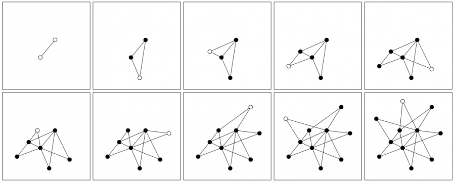
Image 5.3
Evolution of the Barabási-Albert Model
The sequence of images shows nine subsequent steps of the Barabási-Albert model. Empty circles mark the newly added node to the network, which decides where to connect its two links (m=2) using preferential attachment (5.1). After [9].
After t timesteps the Barabási-Albert model generates a network with N = t + m0 nodes and m0 + mt links. As Image 5.4 shows, the obtained network has a power-law degree distribution with degree exponent γ=3. A mathematically self-consistent definition of the model is provided in BOX 5.1.
As Image 5.3 and Video 5.2 indicate, while most nodes in the network have only a few links, a few gradually turn into hubs. These hubs are the result of a rich-gets-richer phenomenon: Due to preferential attachment new nodes are more likely to connect to the more connected nodes than to the smaller nodes. Hence, the larger nodes will acquire links at the expense of the smaller nodes, eventually becoming hubs.
Video 5.2 Emergence of a Scale-free Network
Watch a video that shows the growth of a scale-free network and the emergence of the hubs in the Barabási-Albert model. Courtesy of Dashun Wang.
In summary, the Barabási-Albert model indicates that two simple mechanisms, growth and preferential attachment, are responsible for the emergence of scale-free networks. The origin of the power law and the associated hubs is a rich-gets-richer phenomenon induced by the coexistence of these two ingredients. To understand the model’s behavior and to quantify the emergence of the scale-free property, we need to become familiar with the model’s mathematical properties, which is the subject of the next section.
Image 5.4
The Degree Distribution
The degree distribution of a network generated by the Barabási-Albert model. The figure shows pk for a single network of size N=100,000 and m=3. It shows both the linearly-binned (purple) and the log-binned version (green) of pk. The straight line is added to guide the eye and has slope γ=3, corresponding to the network’s predicted degree exponent.
Section 5.4
Degree Dynamics
To understand the emergence of the scale-free property, we need to focus on the time evolution of the Barabási-Albert model. We begin by exploring the time-dependent degree of a single node [11].
In the model an existing node can increase its degree each time a new node enters the network. This new node will link to m of the N(t) nodes already present in the system. The probability that one of these links connects to node i is given by (5.1).
Let us approximate the degree ki with a continuous real variable, representing its expectation value over many realizations of the growth process. The rate at which an existing node i acquires links as a result of new nodes connecting to it is
The coefficient m describes that each new node arrives with m links. Hence, node i has m chances to be chosen. The sum in the denominator of (5.3) goes over all nodes in the network except the newly added node, thus
]
Therefore (5.4) becomes
For large t the (-1) term can be neglected in the denominator, obtaining
By integrating (5.6) and using the fact that ki(ti)=m, meaning that node i joins the network at time ti with m links, we obtain
We call β the dynamical exponent and has the value
Equation (5.7) offers a number of predictions:
The degree of each node increases following a power-law with the same dynamical exponent β =1/2 (Image 5.6a). Hence all nodes follow the same dynamical law.
The growth in the degrees is sublinear (i.e. β < 1). This is a consequence of the growing nature of the Barabási-Albert model: Each new node has more nodes to link to than the previous node. Hence, with time the existing nodes compete for links with an increasing pool of other nodes.
The earlier node i was added, the higher is its degree ki(t). Hence, hubs are large because they arrived earlier, a phenomenon called first-mover advantage in marketing and business.
The rate at which the node i acquires new links is given by the derivative of (5.7)
indicating that in each time step older nodes acquire more links (as they have smaller ti). Furthermore the rate at which a node acquires links decreases with time as t−1/2. Hence, fewer and fewer links go to a node.
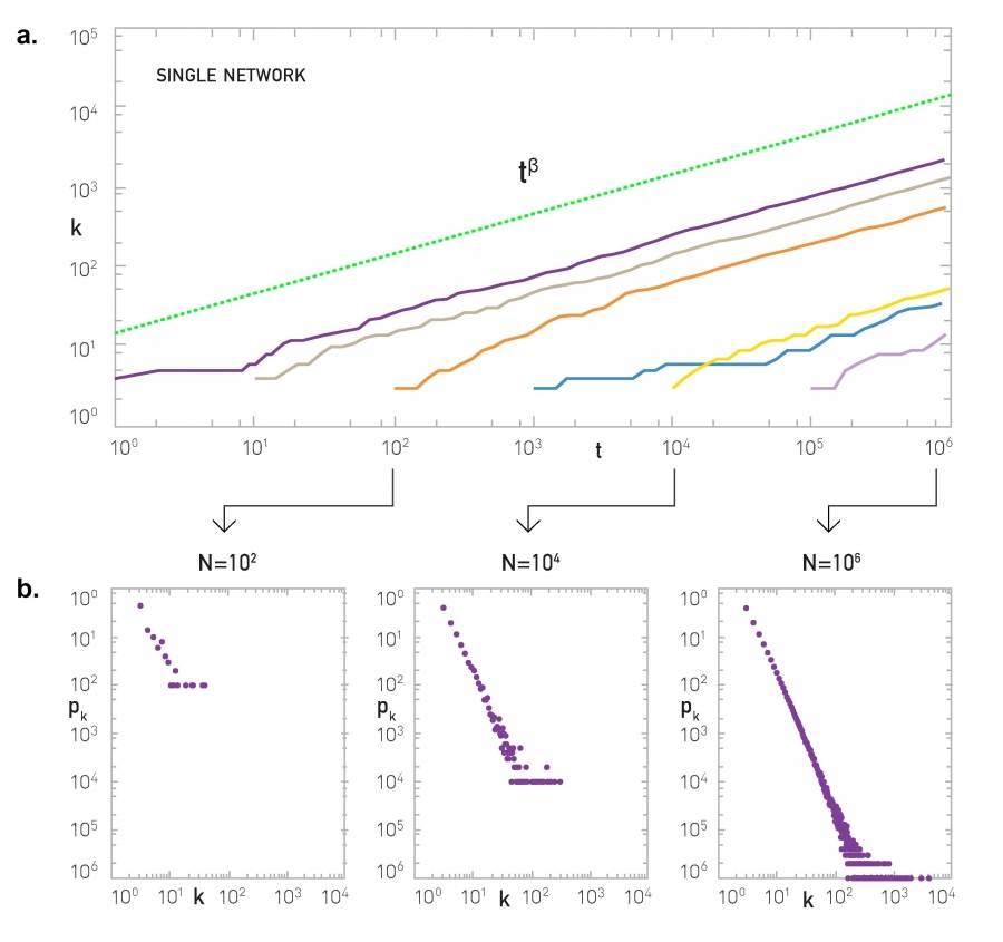
Image 5.6
Degree Dynamics
The growth of the degrees of nodes added at time t =1, 10, 102, 103, 104, 105 (continuous lines from left to right) in the Barabási-Albert model. Each node increases its degree following (5.7). Consequently at any moment the older nodes have higher degrees. The dotted line corresponds to the analytical prediction (5.7) with β = 1/2.
Degree distribution of the network after adding N = 102, 104, and 106 nodes, i.e. at time t = 102, 104, and 106 (illustrated by arrows in (a)). The larger the network, the more obvious is the power-law nature of the degree distribution. Note that we used linear binning for pk to better observe the gradual emergence of the scale-free state.
In summary, the Barabási-Albert model captures the fact that in real networks nodes arrive one after the other, offering a dynamical description of a network’s evolution. This generates a competition for links during which the older nodes have an advantage over the younger ones, eventually turning into hubs.
Section 5.5
Degree Distribution
The distinguishing feature of the networks generated by the Barabási- Albert model is their power-law degree distribution (Image 5.4). In this section we calculate the functional form of pk, helping us understand its origin.
A number of analytical tools are available to calculate the degree distribution of the Barabási-Albert network. The simplest is the continuum theory that we started developing in the previous section [1, 11]. It predicts the degree distribution (BOX 5.3),
with
Therefore the degree distribution follows a power law with degree exponent γ=3, in agreement with the numerical results (Figures 5.4 and 5.7). Moreover (5.10) links the degree exponent, γ, a quantity characterizing the network topology, to the dynamical exponent β that characterizes a node’s temporal evolution, revealing a deep relationship between the network's topology and dynamics.
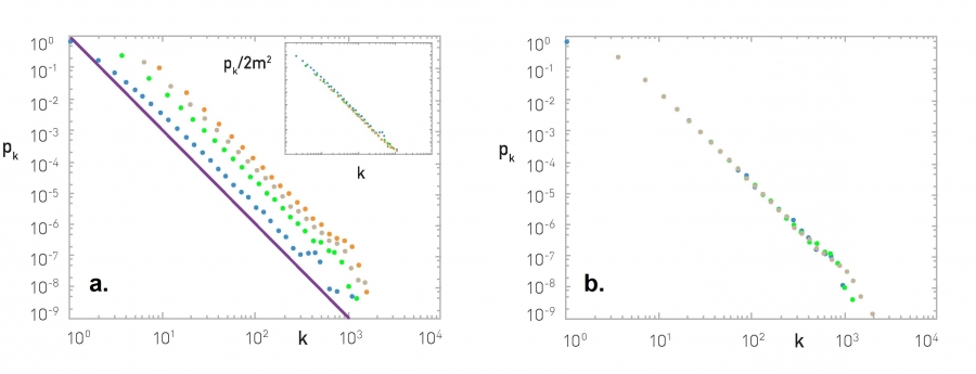
Image 5.7
Probing the Analytical Predictions
We generated networks with N=100,000 and m0=m=1 (blue), 3 (green), 5 (grey), and 7 (orange). The fact that the curves are parallel to each other indicates that γ is independent of m and m0. The slope of the purple line is -3, corresponding to the predicted degree exponent γ=3. Inset: (5.11) predicts pk~2m2, hence pk/2m2 should be independent of m. Indeed, by plotting pk/2m2 vs. k, the data points shown in the main plot collapse into a single curve.
The Barabási-Albert model predicts that pk is independent of N. To test this we plot pk for N = 50,000 (blue), 100,000 (green), and 200,000 (grey), with m0=m=3. The obtained pk are practically indistinguishable, indicating that the degree distribution is stationary, i.e. independent of time and system size.
While the continuum theory predicts the correct degree exponent, it fails to accurately predict the pre-factors of (5.9). The correct pre-factors can be obtained using a master [12] or rate equation [13] approach or calculated exactly using the LCD model [10] (BOX 5.3). Consequently the exact degree distribution of the Barabási-Albert model is (ADVANCED TOPICS 5.A)
Equation (5.11) has several implications:
For large k (5.11) reduces to pk~ k-3, or γ = 3, in line with (5.9) and (5.10).
The degree exponent γ is independent of m, a prediction that agrees with the numerical results (Image 5.7a).
The power-law degree distribution observed in real networks describes systems of rather different age and size. Hence, an approriate model should lead to a time-independent degree distribution. Indeed, according to (5.11) the degree distribution of the Barabási-Albert model is independent of both t and N. Hence the model predicts the emergence of a stationary scale-free state. Numerical simulations support this prediction, indicating that pk observed for different t (or N) fully overlap (Image 5.7b).
Equation (5.11) predicts that the coefficient of the power-law distribution is proportional to m(m + 1) (or m2 for large m), again confirmed by numerical simulations (Image 5.7a, inset).
In summary, the analytical calculations predict that the Barabási-Albert model generates a scale-free network with degree exponent γ=3. The degree exponent is independent of the m and m0 parameters. Furthermore, the degree distribution is stationary (i.e. time invariant), explaining why networks with different history, size and age develop a similar degree distribution.
Section 5.6
The Absence of Growth or Preferential Attachment
The coexistence of growth and preferential attachment in the Barabási- Albert model raises an important question: Are they both necessary for the emergence of the scale-free property? In other words, could we generate a scale-free network with only one of the two ingredients? To address these questions, next we discuss two limiting cases of the model, each containing only one of the two ingredients [1, 11].
Model A
To test the role of preferential attachment we keep the growing character of the network (ingredient A) and eliminate preferential attachment (ingredient B). Hence, Model A starts with m0 nodes and evolves following these steps:
Growth
At each time step we add a new node with m(≤m0) links that connect to m nodes added earlier.
Preferential Attachment
The probability that a new node links to a node with degree ki is
That is, Π(ki) is independent of ki, indicating that new nodes choose randomly the nodes they link to.
Image 5.8
Model A and Model B
Numerical simulations probing the role of growth and preferential attachment.
Model A
Degree distribution for Model A, that incorporates growth but lacks preferential attachment. The symbols correspond to m0=m=1 (circles), 3 (squares), 5 diamonds), 7 (triangles) and N=800,000. The linear-log plot indicates that the resulting network has an exponential pk, as predicted by (5.18).
Inset: Time evolution of the degree of two nodes added at t1=7 and t2=97 for m0=m=3. The dashed line follows (5.17).
Model B
Degree distribution for Model B, that lacks growth but incorporates preferential attachment, shown for N=10,000 and t=N (circles), t=5N (squares), and t=40N (diamonds). The changing shape of pk indicates that the degree distribution is not stationary.
Inset: Time dependent degrees of two nodes (N=10,000), indicating that ki(t) grows linearly, as predicted by (5.19). After [11].
The continuum theory predicts that for Model A ki(t) increases logarithmically with time
a much slower growth than the power law increase (5.7). Consequently the degree distribution follows an exponential (Image 5.8a)
An exponential function decays much faster than a power law, hence it does not support hubs. Therefore the lack of preferential attachment eliminates the network’s scale-free character and the hubs. Indeed, as all nodes acquire links with equal probabilty, we lack a rich-get-richer process and no clear winner can emerge.
Model B
To test the role of growth next we keep preferential attachment (ingredient B) and eliminate growth (ingredient A). Hence, Model B starts with N nodes and evolves following this step:
Preferential Attachment
At each time step a node is selected randomly and connected to node i with degree ki already present in the network, where i is chosen with probability Π(k). As Π(0)=0 nodes with k=0 are assumed to have k=1, otherwise they can not acquire links.
In Model B the number of nodes remains constant during the network’s evolution, while the number of links increases linearly with time. As a result for large t the degree of each node also increases linearly with time (Image 5.7b, inset)
Indeed, in each time step we add a new link, without changing the number of nodes.
At early times, when there are only a few links in the network (i.e. L ≪ N), each new link connects previously unconnected nodes. In this stage the model’s evolution is indistinguishable from the Barabási-Albert model with m=1. Numerical simulations show that in this regime the model develops a degree distribution with a power-law tail (Image 5.8b).
Yet, pk is not stationary. Indeed, after a transient period the node degrees converge to the average degree (5.19) and the degree develops a peak (Image 5.8b). For t → N(N-1)/2 the network becomes a complete graph in which all nodes have degree kmax=N-1, hence pk= δ(N-1).
In summary, the absence of preferential attachment leads to a growing network with a stationary but exponential degree distribution. In contrast the absence of growth leads to the loss of stationarity, forcing the network to converge to a complete graph. This failure of Models A and B to reproduce the empirically observed scale-free distribution indicates that growth and preferential attachment are simultaneously needed for the emergence of the scale-free property.
Section 5.7
Measuring Preferential Attachment
In the previous section we showed that growth and preferential attachment are jointly responsible for the scale-free property. The presence of growth in real systems is obvious: All large networks have reached their current size by adding new nodes. But to convince ourselves that preferential attachment is also present in real networks, we need to detect it experimentally. In this section we show how to detect preferential attachment by measuring the Π(k) function in real networks.
Preferential attachment relies on two distinct hypotheses:
Hypothesis 1
The likelihood to connect to a node depends on that node’s degree k. This is in contrast with the random network model, for which Π(k) is independent of k.
Hypothesis 2
The functional form of Π(k) is linear in k.
Both hypotheses can be tested by measuring Π(k). We can determine Π(k) for systems for which we know the time at which each node joined the network, or we have at least two network maps collected at not too distant moments in time [14, 15].
Consider a network for which we have two different maps, the first taken at time t and the second at time t + Δt (Image 5.9a). For nodes that changed their degree during the Δt time frame we measure Δki = ki(t+Δt )−ki(t). According to (5.1), the relative change Δki/Δt should follow
providing the functional form of preferential attachment. For (5.20) to be valid we must keep Δt small, so that the changes in Δk are modest. But Δt must not be too small so that there are still detectable differences between the two networks.
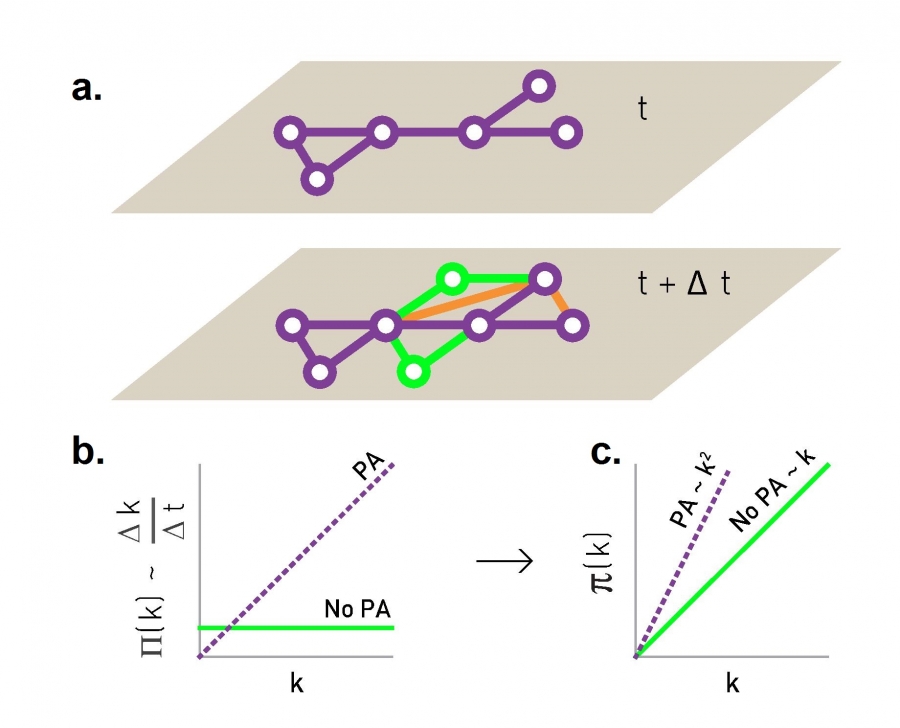
Image 5.9
Detecting Preferential Attachment
If we have access to two maps of the same network taken at time t and t+Δt, comparing them allows us to measure the Π(k) function. Specifically, we look at nodes that have gained new links thanks to the arrival of the two new green nodes at t+Δt. The orange lines correspond to links that connect previously disconnected nodes, called internal links. Their role is discussed in CHAPTER 6.
In the presence of preferential attachment Δk/Δt will depend linearly on a node’s degree at time t.
The scaling of the cumulative preferential attachment function π(k) helps us detect the presence or absence of preferential attachment (Image 5.10).
In practice the obtained Δki/Δt curve can be noisy. To reduce this noise we measure the cumulative preferential attachment function
In the absence of preferential attachment we have Π(ki)=constant, hence, π(k) ~ k according to (5.21). If linear preferential attachment is present, i.e. if Π(ki)=ki, we expect π(k) ~ k2.
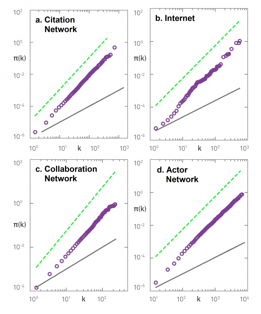
Image 5.10 shows the measured π(k) for four real networks. For each system we observe a faster than linear increase in π(k), indicating the presence of preferential attachment. Image 5.10 also suggests that Π(k) can be approximated with
For the Internet and citation networks we have α ≈ 1, indicating that Π(k) depends linearly on k, following (5.1). This is in line with Hypotheses 1 and 2. For the co-authorship and the actor network the best fit provides α=0.9±0.1 indicating the presence of a sublinear preferential attachment.
In summary, (5.20) allows us to detect the presence (or absence) of preferential attachment in real networks. The measurements show that the attachment probability depends on the node degree. We also find that while in some systems preferential attachment is linear, in others it can be sublinear. The implications of this non-linearity are discussed in the next section.
Image 5.10
Evidence of Preferential Attachmentt
The figure shows the cumulative preferential attachment function π(k), defined in (5.21), for several real systems:
Citation network.
Internet.
Scientific collaboration network (neuroscience).
Actor network.
In each panel we have two lines to guide the eye: The dashed line corresponds to linear preferential attachment (π(k)~k2) and the continuous line indicates the absence of preferential attachment (π(k)~k). In line with Hypothesis 1 we detect a k-dependence in each dataset. Yet, in (c) and (d) π(k) grows slower than k2, indicating that for these systems preferential attachment is sublinear, violating Hypothesis 2. Note that these measurements only consider links added through the arrival of new nodes, ignoring the addition of internal links. After [14].
Section 5.8
Non-linear Preferential Attachment
The observation of sublinear preferential attachment in Image 5.10 raises an important question: What is the impact of this nonlinearity on the network topology? To answer this we replace the linear preferential attachment (5.1) with (5.22) and calculate the degree distribution of the obtained nonlinear Barabási-Albert model.
The behavior for α=0 is clear: In the absence of preferential attachment we are back to Model A discussed in SECTION 5.4. Consequently the degree distribution follows the exponential (5.17).
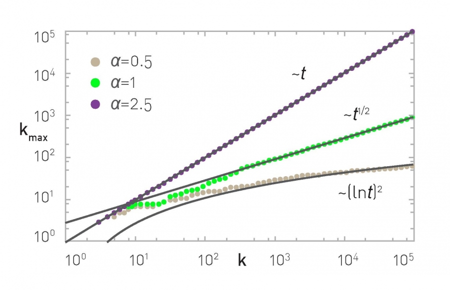
Image 5.11
The Growth of the Hubs
The nature of preferential attachment affects the degree of the largest node. While in a scalefree network (α=1) the biggest hub grows as t1/2 (green curve, (4.18)), for sublinear preferential attachment (α < 1) this dependence becomes logarithmic, following (5.24). For superlinear preferential attachment (α > 1) the biggest hub grows linearly with time, always grabbing a finite fraction of all links, following (5.25). The symbols are provided by numerical simulations; the dotted lines represent the analytical predictions.
For α = 1 we recover the Barabási-Albert model, obtaining a scale-free network with degree distribution (5.14).
Next we focus on the case α ≠ 0 and α ≠ 1. The calculation of pk for an arbitrary α predicts several scaling regimes [13] (ADVANCED TOPICS 5.B):
Sublinear Preferential Attachment (0 < α < 1)
For any α > 0 new nodes favor the more connected nodes over the less connected nodes. Yet, for α < 1 the bias is weak, not sufficient to generate a scale-free degree distribution. Instead, in this regime the degrees follow the stretched exponential distribution (SECTION 4.10)
where μ(α) depends only weakly on α. The exponential cutoff in (5.23) implies that sublinear preferential attachment limits the size and the number of the hubs.
Sublinear preferential attachment also alters the size of the largest degree, kmax. For a scale-free network kmax scales polynomially with time, following (4.18). For sublinear preferential attachment we have
a logarithmic dependence that predicts a much slower growth of the maximum degee than the polynomial. This slower growth is the reason why the hubs are smaller for α < 1 (Image 5.11).
Superlinear Preferential Attachment (α > 1)
For α > 1 the tendency to link to highly connected nodes is enhanced, accelerating the rich-gets-richer process. The consequence of this is most obvious for α > 2, when the model predicts a winner-takes-all phenomenon: almost all nodes connect to a few super-hubs. Hence we observe the emergence of a hub-and-spoke network, in which most nodes link directly to a few central nodes. The situation for 1 < α < 2 is less extreme, but similar.
This winner-takes-all process alters the size of the largest hub as well, finding that (Image 5.11).
In summary, nonlinear preferential attachment changes the degree distribution, either limiting the size of the hubs (α < 1), or leading to super- hubs (α > 1, Image 5.12). Consequently, Π(k) needs to depend strictly linearly on the degrees for the resulting network to have a pure power law pk. While in many systems we do observe such a linear dependence, in others, like the scientific collaboration network and the actor network, preferential attachment is sublinear. This nonlinear Π(k) is one reason the degree distribution of real networks deviates from a pure power-law. Hence for systems with sublinear Π(k) the stretched exponential (5.23) should offer a better fit to the degree distribution.
Image 5.12
Nonlinear Preferential Attachment
The scaling regimes characterizing the nonlinear Barabási-Albert model. The three top panels show pk for different α (N=104). The network maps show the corresponding topologies (N=100). The theoretical results predict the existence of four scaling regimes:
No Preferential Attachment (α=0)
The network has a simple exponential degree distribution, following (5.18). Hubs are absent and the resulting network is similar to a random network.
Sublinear Regime (0 < α < 1)
The degree distribution follows the stretched exponential (5.23), resulting in fewer and smaller hubs than in a scale-free network. As α → 1 the cutoff length increases and pk follows a power law over an increasing range of degrees.
Linear Regime (α=1)
This corresponds to the Barabási-Albert model, hence the degree distribution follows a power law.
Superlinear Regime (α > 1)
The high-degree nodes are disproportionately attractive. A winner-takes-all dynamics leads to a hub-and-spoke topology. In this configuration the earliest nodes become super hubs and all subsequent nodes link to them. The degree distribution, shown for α=1.5 indicates the coexistence of many small nodes with a few super hubs in the vicinity of k=104.
Section 5.9
The Origins of Preferential Attachment
Given the key role preferential attachment plays in the evolution of real networks, we must ask, where does it come from? The question can be broken to two narrower issues:
Why does Π(k) depend on k?
Why is the dependence of Π(k) linear in k?
In the past decade we witnessed the emergence of two philosophically different answers to these questions. The first views preferential attachment as the interplay between random events and some structural property of a network. These mechanisms do not require global knowledge of the network but rely on random events, hence we will call them local or random mechanisms. The second assumes that each new node or link balances conflicting needs, hence they are preceeded by a cost-benefit analysis. These models assume familiarity with the whole network and rely on optimization principles, prompting us to call them global or optimized mechanisms. In this section we discuss both approaches.
Local Mechanisms
The Barabási-Albert model postulates the presence of preferential attachment. Yet, as we show below, we can build models that generate scalefree networks apparently without preferential attachment. They work by generating preferential attachment. Next we discuss two such models and derive Π(k) for them, allowing us to understand the origins of preferential attachment.
Image 5.13
Link Selection Model
The network grows by adding a new node, that selects randomly a link from the network (shown in purple).
The new node connects with equal probability to one of the two nodes at the ends of the selected link. In this case the new node connected to the node at the right end of the selected link.
Link Selection Model
The link selection model offers perhaps the simplest example of a local mechanism that generates a scale-free network without preferential attachment [16]. It is defined as follows (Image 5.13):
Growth: At each time step we add a new node to the network.
Link Selection: We select a link at random and connect the new node to one of the two nodes at the two ends of the selected link. The model requires no knowledge about the overall network topology, hence it is inherently local and random. Unlike the Barabási-Albert model, it lacks a built-in Π(k) function. Yet, next we show that it generates preferential attachment.
We start by writing the probability qk that the node at the end of a randomly chosen link has degree k as
Equation (5.26) captures two effects:
The higher is the degree of a node, the higher is the chance that it is located at the end of the chosen link.
The more degree-k nodes are in the network (i.e., the higher is pk), the more likely that a degree k node is at the end of the link.
In (5.26) C can be calculated using the normalization condition Σqk = 1, obtaining C=1/〈k〉. Hence the probability to find a degree-k node at the end of a randomly chosen link is
Equation (5.27) is the probability that a new node connects to a node with degree k. The fact that the bias in (5.27) is linear in k indicates that the link selection model builds a scale-free network by generating linear preferential attachment.
Copying Model
While the link selection model offers the simplest mechanism for preferential attachment, it is neither the first nor the most popular in the class of models that rely on local mechanisms. That distinction goes to the copying model (Image 5.14). The model mimics a simple phenomena: The authors of a new webpage tend to borrow links from other webpages on related topics [17, 18]. It is defined as follows:
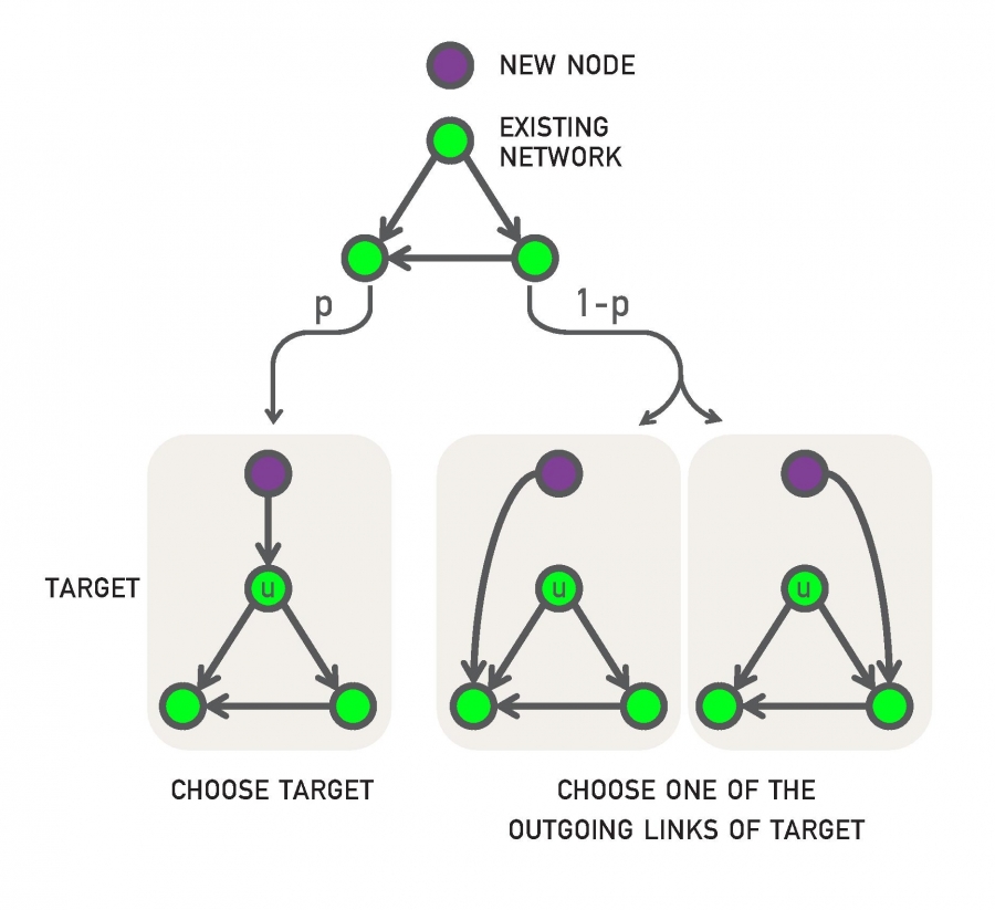
Image 5.14
Copying Model
The main steps of the copying model. A new node connects with probability p to a randomly chosen target node u, or with probability 1-p to one of the nodes the target u points to. In other words, with probabilty 1-p the new node copies a link of its target u.
In each time step a new node is added to the network. To decide where it connects we randomly select a node u, corresponding for example to a web document whose content is related to the content of the new node. Then we follow a two-step procedure (Image 5.14):
Random Connection: With probability p the new node links to u, which means that we link to the randomly selected web document.
Copying: With probability 1-p we randomly choose an outgoing link of node u and link the new node to the link’s target. In other words, the new webpage copies a link of node u and connects to its target, rather than connecting to node u directly.
The probability of selecting a particular node in step (i) is 1/N. Step (ii) is equivalent with selecting a node linked to a randomly selected link. The probability of selecting a degree-k node through this copying step (ii) is k/2L for undirected networks. Combining (i) and (ii), the likelihood that a new node connects to a degree-k node follows
which, being linear in k, predicts a linear preferential attachment
The popularity of the copying model lies in its relevance to real systems:
Social Networks: The more acquaintances an individual has, the higher is the chance that she will be introduced to new individuals by her existing acquaintances. In other words, we "copy" the friends of our friends. Consequently without friends, it is difficult to make new friends.
Citation Networks: No scientist can be familiar with all papers published on a certain topic. Authors decide what to read and cite by "copying" references from the papers they have read. Consequently papers with more citations are more likely to be studied and cited again.
Protein Interactions: Gene duplication, responsible for the emergence of new genes in a cell, can be mapped into the copying model, explaining the scale-free nature of protein interaction networks [19, 20].
Taken together, we find that both the link selection model and the copying model generate a linear preferential attachment through random linking.
Optimization
A longstanding assumption of economics is that humans make rational decisions, balancing cost against benefits. In other words, each individual aims to maximize its personal advantage. This is the starting point of rational choice theory in economics [21] and it is a hypothesis central to modern political science, sociology, and philosophy. As we show below, such rational decisions can lead to preferential attachment [22, 23, 24].
Consider the Internet, whose nodes are routers connected via cables. Establishing a new Internet connection between two routers requires us to lay down a new cable between them. As this is costly, each new link is preceded by a careful cost-benefit analysis. Each new router (node) will choose its link to balance access to good network performance (i.e. proper bandwith) with the cost of laying down a new cable (i.e. physical distance). This can be a conflicting desire, as the closest node may not offer the best network performance
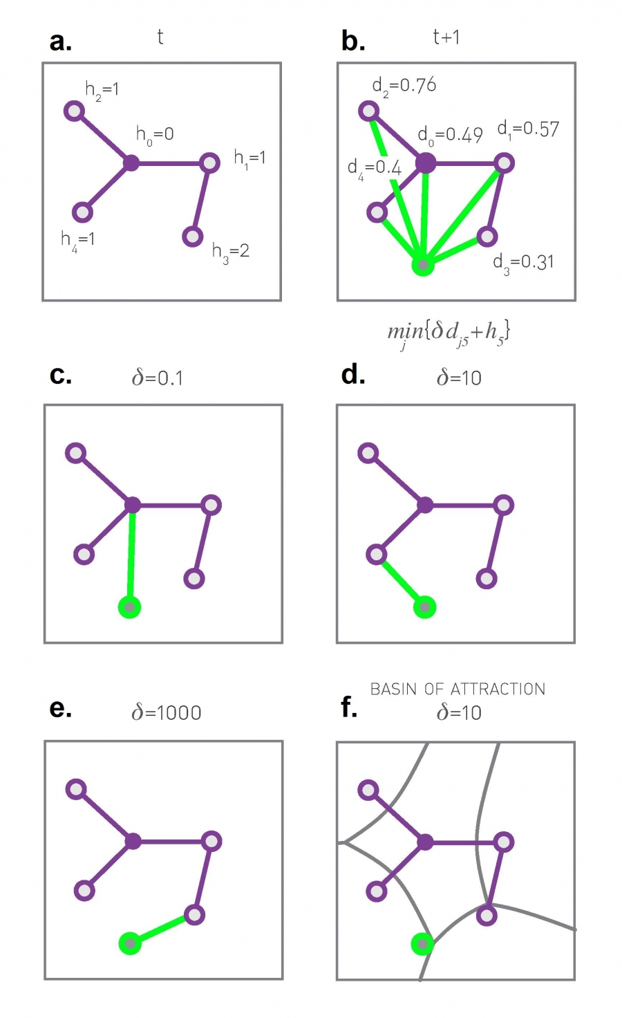
For simplicity let us assume that all nodes are located on a continent with the shape of a unit square. At each time step we add a new node and randomly choose a point within the square as its physical location. When deciding where to connect the new node i, we calculate the cost function [22]
which compares the cost of connecting to each node j already in the network. Here dij is the Euclidean distance between the new node i and the potential target j, and hj is the network-based distance of node j to the first node of the network, which we designate as the desireable “center“ of the network (Image 5.15), offering the best network performance. Hence hj captures the “resources” offered by node j, measured by its distance to the network’s center.
Image 5.15
Optimization Model
(a)A small network, where the hj term in the cost function (5.28) is shown for each node. Here hj represents the network-based distance of node j from node i=0, designated as the "center" of the network, offering the best network performance. Hence h0=0 and h3=2.
(b)A new node (green) will choose the node j to which it connects by minimizing Cj of (5.28).
(c)-(e) If δ is small the new node will connect to the central node with hj =0. As we increase δ, the balance in (5.28) shifts, forcing the new node to connect to more distant nodes. The panels (c)-(e) show the choice of the new green node makes for different values of δ.
(f) The basin of attraction for each node for δ=10. A new node arriving inside a basin will always link to the node at the center of the basin. The size of each basin depends on the degree of the node at its center. Indeed, the smaller is hj, the larger can be the distance to the new node while still minimizing (5.28). Yet, the higher is the degree of node j, the smaller is its expected distance to the central node hj.
The calculations indicate the emergence of three distinct network topologies, depending on the value of the parameter δ in (5.28) and N (Image 5.15):
Star Network δ < (1/2)1/2
For δ = 0 the Euclidean distances are irrelevant, hence each node links to the central node, turning the network into a star. We have a star configuration each time when the hj term dominates over δdij in (5.28).
Random Network δ ≥ N1/2
For very large δ the contribution provided by the distance term δdij overwhelms hj in (5.28). In this case each new node connects to the node closest to it. The resulting network will have a bounded degree distribution, like a random network (Image 5.16b).
Scale-free Network 4 ≤ δ ≤ N1/2
Numerical simulations and analytical calculations indicate that for intermediate δ values the network develops a scale-free topology [22]. The origin of the power law distribution in this regime is rooted in two competing mechanisms:
Optimization: Each node has a basin of attraction, so that nodes landing in this basin will always link to it. The size of each basin correlates with hj of node j at its center, which in turn correlates with the node’s degree kj (Image 5.15f).
Randomness: We choose randomly the location of the new node, ending in one of the N basins of attraction. The node with the largest degree has largest basin of attraction, hence gains the most new nodes and links. This leads to preferential attachment, as documented in Image 5.16d.
Image 5.16
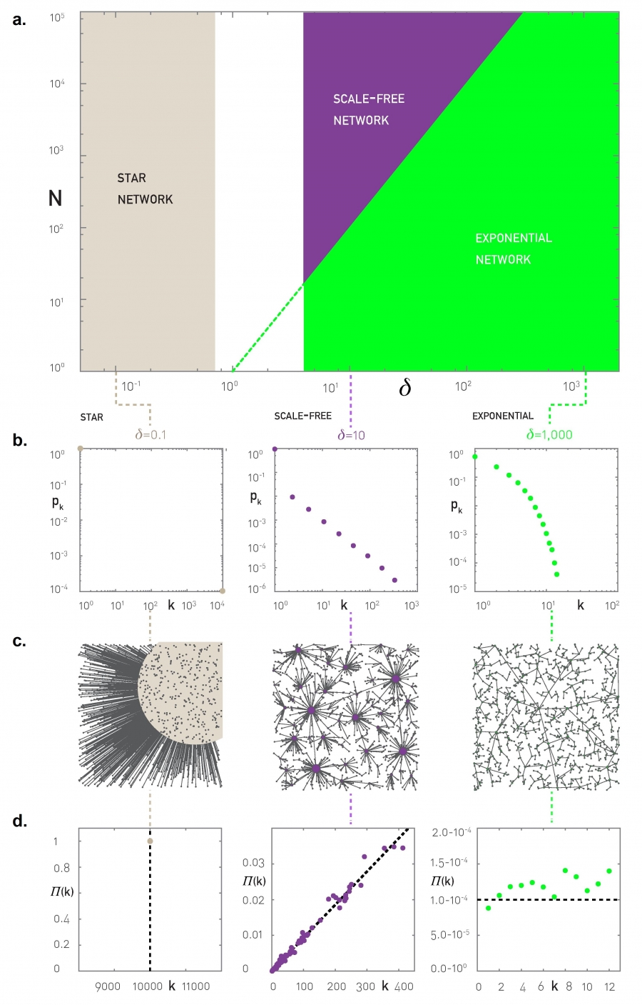
Scaling in the Optimization Model
The three network classes generated by the optimization model: star, scale-free, and exponential networks. The topology of the network in the unmarked area is unknown.
The vertical boundary of the star configuration is at δ=(1/2)1/2. This is the inverse of the maximum distance between two nodes on a square lattice with unit length, over which the model is defined. Therefore if δ < (1/2)1/2, for any new node δdij< 1 and the cost (5.28) of connecting to the central node is Ci = δdij+0, always lower than connecting to any other node at the cost of f(i,j) = δdij+1. Therefore for δ < (1/2)1/2 all nodes connect to node 0, resulting in a network dominated by a single hub (starand-spoke network (c)).
The oblique boundary of the scale-free regime is δ = N1/2. Indeed, if nodes are placed randomly on the unit square, then the typical distance between neighbors decreases as N−1/2. Hence, if dij~N−1/2 then δdij≥hij for most node pairs. Typically the path length to the central node hj grows slower than N (in small-world networks hj~log N, in scale-free networks hj~lnlnN). Therefore Ci is dominated by the δdij term and the smallest Ci is achieved by minimizing the distance-dependent term. Note that strictly speaking the transition only occurs in the N → ∞ limit. In the white regime we lack an analytical form for the degree distribution.
Degree distribution of networks generated in the three phases marked in (a) for N=104.
Typical topologies generated by the optimization model for selected δ values. Node size is proportional to its degree.
We used the method described in SECTION 5.6 to measure the preferential attachment function. Starting from a network with N=10,000 nodes we added a new node and measured the degree of the node that it connected to. We repeated this procedure 10,000 times, obtaining Π(k). The plots document the presence of linear preferential attachment in the scale-free phase, but its absence in the star and the exponential phases.
In summary, we can build models that do not have an explicit Π(k) function built into their definition, yet they generate a scale-free network. As we showed in this section, these work by inducing preferential attachment. The mechanism responsible for preferential attachment can have two fundamentally different origins (Image 5.17): it can be rooted in random processes, like link selection or copying, or in optimization, when new nodes balance conflicting criteria as they decide where to connect. Note that each of the mechanisms discussed above lead to linear preferential attachment, as assumed in the Barabási-Albert model. We are not aware of mechanisms capable of generating nonlinear preferential attachment, like those discussed in SECTION 5.7.
The diversity of the mechanisms discussed in this section suggest that linear preferential attachment is present in so many and so different systems precisely because it can come from both rational choice and random actions [25]. Most complex systems are driven by processes that have a bit of both. Hence luck or reason, preferential attachment wins either way.
Image 5.17
Luck or Reason: an Ancient Fight
The tension between randomness and optimization, two apparently antagonistic explanations for power laws, is by no means new: In the 1960s Herbert Simon and Benoit Mandelbrot have engaged in a fierce public dispute over this very topic. Simon proposed that preferential attachment is responsible for the power-law nature of word frequencies. Mandelbrot fiercely defended an optimization-based framework. The debate spanned seven papers and two years and is one of the most vicious scientific disagreement on record.
In the context of networks today the argument titled in Simon’s favor: The power laws observed in complex networks appear to be driven by randomness and preferential attachment. Yet, the optimization-based ideas proposed by Mandelbrot play an important role in explaining the origins of preferential attachment. So at the end they were both right.
Section 5.10
Diameter and Clustering Coefficient
To complete the characterization of the Barabási-Albert model we discuss the behavior of the network diameter and the clustering coefficient.
Diameter
The network diameter, representing the maximum distance in the Barabási-Albert network, follows for m > 1 and large N [33, 34]
Therefore the diameter grows slower than ln N, making the distances in the Barabási-Albert model smaller than the distances observed in a random graph of similar size. The difference is particularly relevant for large N.
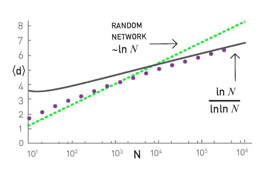
Note that while (5.29) is derived for the diameter, the average distance 〈d〉 scales in a similar fashion. Indeed, as we show in Image 5.18, for small N the ln N term captures the scaling of 〈d〉 with N, but for large N(≥104) the impact of the logarithmic correction ln ln N becomes noticeable.
Image 5.18
Average Distance
The dependence of the average distance on the system size in the Barabási-Albert model. The continuous line corresponds to the exact result (5.29), while the dotted line corresponds to the prediction (3.19) for a random network. The analytical predictions do not provide the exact perfactors, hence the lines are not fits, but indicate only the predicted N-dependent trends. The results were averaged for ten independent runs for m = 2.
Clustering coefficient
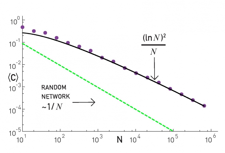
The clustering coefficient of the Barabási-Albert model follows (ADVANCED TOPICS 5.C) [35, 36]
The prediction (5.30) is quite different from the 1/N dependence obtained for the random network model (Image 5.19). The difference comes in the (lnN)2 term, that increases the clustering coefficient for large N. Consequently the Barabási-Albert network is locally more clustered than a random network.
Image 5.19
Clustering Coefficient
The dependence of the average clustering coefficient on the system size N for the Barabási-Albert model. The continuous line corresponds to the analytical prediction (5.30), while the dotted line corresponds to the prediction for a random network, for which 〈C〉 ~ 1/N. The results are averaged for ten independent runs for m = 2. The dashed and continuous curves are not fits, but are drawn to indicate the predicted N dependent trends.
Section 5.11
Summary
The most important message of the Barabási-Albert model is that network structure and evolution are inseparable. Indeed, in the Erdős-Rényi, Watts-Strogatz, the configuration and the hidden parameter models the role of the modeler is to cleverly place the links between a fixed number of nodes. Returning to our earlier analogy, the networks generated by these models relate to real networks like a photo of a painting relates to the painting itself: It may look like the real one, but the process of generating a photo is drastically different from the process of painting the original painting. The aim of the Barabási-Albert model is to capture the processes that assemble a network in the first place. Hence, it aims to paint the painting again, coming as close as possible to the original brush strokes. Consequently, the modeling philosophy behind the model is simple: to understand the topology of a complex system, we need to describe how it came into being.
Random networks, the configuration and the hidden parameter models will continue to play an important role as we explore how certain network characteristics deviate from our expectations. Yet, if we want to explain the origin of a particular network property, we will have to use models that capture the system’s genesis.
The Barabási-Albert model raises a fundamental question: Is the combination of growth and preferential attachment the real reason why networks are scale-free? We offered a necessary and sufficient argument to address this question. First, we showed that growth and preferential attachment are jointly needed to generate scale-free networks, hence if one of them is absent, either the scale-free property or stationarity is lost. Second, we showed that if they are both present, they do lead to scale-free networks. This argument leaves one possibility open, however: Do these two mechanisms explain the scale-free nature of all networks? Could there be some real networks that are scale-free thanks to some completely different mechanism? The answer is provided in SECTION 5.9, where we did encountered the link selection, the copying and the optimization models that do not have a preferential attachment function built into them, yet they do lead to a scale-free network. We showed that they do so by generating a linear Π(k). This finding underscores a more general pattern: To date all known models and real systems that are scale-free have been found to have preferential attachment. Hence the basic mechanisms of the Barabási-Albert model appear to capture the origin of their scale-free topology.
The Barabási-Albert model is unable to describe many characteristics of real systems:
The model predicts γ=3 while the degree exponent of real networks varies between 2 and 5 (Table 4.2).
Many networks, like the WWW or citation networks, are directed, while the model generates undirected networks.
Many processes observed in networks, from linking to already existing nodes to the disappearance of links and nodes, are absent from the model.
The model does not allow us to distinguish between nodes based on some intrinsic characteristics, like the novelty of a research paper or the utility of a webpage.
While the Barabási-Albert model is occasionally used as a model of the Internet or the cell, in reality it is not designed to capture the details of any particular real network. It is a minimal, proof of principle model whose main purpose is to capture the basic mechanisms responsible for the emergence of the scale-free property. Therefore, if we want to understand the evolution of systems like the Internet, the cell or the WWW, we need to incorporate the important details that contribute to the time evolution of these systems, like the directed nature of the WWW, the possibility of internal links and node and link removal.
As we show in CHAPTER 6, these limitations can be systematically resolved.
Section 5.12
Homework
Generating Barabási-Albert Networks
With the help of a computer, generate a network with N = 104 nodes using the Barabási-Albert model with m = 4. Use as initial condition a fully connected network with m = 4 nodes.
Measure the degree distribution at intermediate steps, namely when the network has 102, 103 and 104 nodes.
Compare the distributions at these intermediate steps by plotting them together and fitting each to a power-law with degree exponent γ. Do the distributions "converge"?
Plot together the cumulative degree distributions at intermediate steps.
Measure the average clustering coefficient in function of N.
Following Image 5.6a, measure the degree dynamics of one of the initial nodes and of the nodes added to the network at time t = 100, t = 1,000 and t = 5,000.
Directed Barabási-Albert Model
Consider a variation of the Barabási-Albert model, where at each time step a new node arrives and connects with a directed link to a node chosen with probability
Here kiin indicates the in-degree of node i and A is the same constant for all nodes. Each new node has m directed links.
Calculate, using the rate equation approach, the in- and out-degree distribution of the resulting network.
By using the properties of the Gamma and Beta functions, can you find a power-law scaling for the in-degree distribution?
For A = 0 the scaling exponent of the in-degree distribution is different from γ = 3, the exponent of the Barabási-Albert model. Why?
Copying Model
Use the rate equation approach to show that the directed copying model leads to a scale-free network with incoming degree exponent
Growth Without Preferential Attachment
Derive the degree distribution (5.18) of Model A, when a network grows by new nodes connecting randomly to m previously existing nodes. With the help of a computer, generate a network of 104 nodes using Model A. Measure the degree distribution and check that it is consistent with the prediction (5.18).
Section 5.13
Advanced Topic 4.A Deriving the Degree Distribution
A number of analytical techniques are available to calculate the exact form of the degree exponent (5.11). Next we derive it using the rate equation approach [12, 13]. The method is sufficiently general to help explore the properties of a wide range of growing networks. Consequently, the calculations described here are of direct relevance for many systems, from models pertaining to the WWW [16, 17, 18] to describing the evolution of the protein interaction network via gene duplication [19, 20].
Let us denote with N(k,t) the number of nodes with degree k at time t. The degree distribution pk(t) relates to this quantity via pk(t) = N(k,t)/N(t). Since at each time-step we add a new node to the network, we have N = t. That is, at any moment the total number of nodes equals the number of timesteps (BOX 5.2).
We write preferential attachment as
where the 2m term captures the fact that in an undirected network each link contributes to the degree of two nodes. Our goal is to calculate the changes in the number of nodes with degree k after a new node is added to the network. For this we inspect the two events that alter N(k,t) and pk(t) following the arrival of a new node:
A new node can link to a degree-k node, turning it into a degree (k+1) node, hence decreasing N(k,t).
A new node can link to a degree (k-1) node, turning it into a degree k node, hence increasing N(k,t).
The number of links that are expected to connect to degree k nodes after the arrival of a new node is
In (5.32) the first term on the l.h.s. captures the probability that the new node will link to a degree-k node (preferential attachment); the second term provides the total number of nodes with degree k, as the more nodes are in this category, the higher the chance that a new node will attach to one of them; the third term is the degree of the incoming node, as the higher is m, the higher is the chance that the new node will link to a degree-k node. We next apply (5.32) to cases (i) and (ii) above:
The number of degree k nodes that acquire a new link and turn into (k+1) degree nodes is
The number of degree (k-1) nodes that acquire a new link, increasing their degree to k is
Combining (5.33) and (5.34) we obtain the expected number of degree-k nodes after the addition of a new node
This equation applies to all nodes with degree k > m. As we lack nodes with degree k=0,1, ... , m-1 in the network (each new node arrives with degree m) we need a separate equation for degree-m modes. Following the same arguments we used to derive (5.35), we obtain
Equations (5.35) and (5.36) are the starting point of the recursive process that provides pk. Let us use the fact that we are looking for a stationary degree distribution, an expectation supported by numerical simulations (Image 5.6). This means that in the N = t → ∞ limit, pk(∞)= pk. Using this we can write the l.h.s. of (5.35) and (5.36) as
Therefore the rate equations (5.35) and (5.36) take the form:
Note that (5.37) can be rewritten as
via a k→k+1 variable change.
We use a recursive approach to obtain the degree distribution. That is, we write the degree distribution for the smallest degree, k=m, using (5.38) and then use (5.39) to calculate pk for the higher degrees:
At this point we notice a simple recursive pattern: By replacing in the denomerator m+3 with k we obtain the probability to observe a node with degree k
which represents the exact form of the degree distribution of the Barabási-Albert model.
Note that:
For large k (5.41) becomes pk ~ k-3, in agreement with the numerical result.
The prefactor of (5.11) or (5.41) is different from the prefactor of (5.9).
This form was derived independently in [12] and [13], and the exact mathematical proof of its validity is provided in [10].
Finally, the rate equation formalism offers an elegant continuum equation satisfied by the degree distribution [16]. Starting from the equation
In this section we derive the degree distribution of the nonlinear Barabási-Albert model, governed by the preferential attachment (5.22). We follow Ref. [13], but we adjust the calculation to cover m > 1.
Strictly speaking a stationary degree distribution only exists if α ≤ 1 in (5.22). For α > 1 a few nodes attract a finite fraction of links, as explained in SECTION 5.7, and we do not have a time-independent pk. Therefore we limit ourself to the α ≤ 1 case.
We start with the nonlinear Barabási-Albert model, in which at each time step a new node is added with m new links. We connect each new link to an existing node with probability
where ki is the degree of node i, 0 < α ≤ 1 and
is the normalization factor and t=N(t) represents the number of nodes. Note that μ(0, t)= Σpk (t) =1 and μ(1, t) =Σkkpk (t) =〈k〉=2mt/N is the average degree. Since 0 < α ≤ 1,
Therefore in the long time limit
whose precise value will be calculated later. For simplicity, we adopt the notation μ ≡μ(α ,t → ∞)
Following the rate equation approach introduced in ADVANCED TOPICS 5.A, we write the rate equation for the network’s degree distribution as
The first term on the r.h.s. describes the rate at which nodes with degree (k-1) gain new links; the second term describes the loss of degree-k nodes when they gain new links, turning into (k+1) degree nodes; the last term represents the newly added nodes with degree m.
Asymptotically, in the t→∞ limit, we can write pk=pk(t + 1)=pk(t). Substituting k=m in (5.51) we obtain:
For k > m
Solving (5.53) recursively we obtain
To determine the large k behavior of pk we take the logarithm of (5.57):
Using the series expansion
we obtain
We approximate the sum over j with the integral
which in the special case of nα=1 becomes
Hence we obtain
Consequently the degree distribution has the form
where
The vanishing terms in the exponential do not influence the k → ∞ asymptotic behavior, being relevant only if 1−nα ≥ 1. Consequently pk depends on α as:
That is, for 1/2 < α < 1 the degree distribution follows a stretched exponential. As we lower α, new corrections start contributing each time α becomes smaller than 1/n, where n is an integer.
For α→1 the degree distribution scales as k−3, as expected for the Barabási- Albert model. Indeed for α = 1 we have μ=2, and
Therefore pk ~ k−1exp(−2lnk) = k−3.
Finally we calculate μ (α) =Σjjα pj. For this we write the sum (5.58)
We obtain μ (α) by solving (5.68) numerically.
Section 5.15
Advanced Topic 4.C The Clustering Coefficient
In this section we derive the average clustering coefficient, (5.30), for the Barabási-Albert model. The derivation follows an argument proposed by Klemm and Eguiluz [35], supported by the exact calculation of Bollobás [36].
We aim to calculate the number of triangles expected in the model, which can be linked to the clustering coefficient (SECTION 2.10). We denote the probability to have a link between node i and j with P(i,j). Therefore, the probability that three nodes i, j, l form a triangle is P(i,j)P(i,l)P(j,l). The expected number of triangles in which node l with degree kl participates is thus given by the sum of the probabilities that node l participates in triangles with arbitrary chosen nodes i and j in the network. We can use the continuous degree approximation to write
To proceed we need to calculate P(i,j), which requires us to consider how the Barabási-Albert model evolves. Let us denote the time when node j arrived with tj =j, which we can do as in each time step we added only one new node (event time, BOX 5.2). Hence the probability that at its arrival node j links to node i with degree kiis given by preferential attachment
Using (5.7), we can write
where we used the fact that the arrival time of node j is tj =j and the arrival time of node i is ti = i. Hence (5.70) now becomes
Using this result we calculate the number of triangles in (5.69), writing
The clustering coefficient can be written as
hence we obtain
To simplify (5.74), we note that according to (5.7) we have
which is the degree of node l at time t = N. Hence, for large kl we have
allowing us to write the clustering coefficient of the Barabási-Albert model as
which is independent of l, therefore we obtain the result (5.30).
Section 5.16
Bibliography
[1] A.-L. Barabási and R. Albert. Emergence of scaling in random networks. Science, 286:509-512, 1999.
[2] F. Eggenberger and G. Pólya. Über die Statistik Verketteter Vorgänge. Zeitschrift für Angewandte Mathematik und Mechanik, 3:279-289, 1923.
[3] G.U. Yule. A mathematical theory of evolution, based on the conclusions of Dr. J. C. Willis. Philosophical Transactions of the Royal Society of London. Series B, 213:21-87, 1925.
[4] R. Gibrat. Les Inégalités économiques. Paris, France, 1931.
[5] G. K. Zipf. Human behavior and the principle of least resort. Addison- Wesley Press, Oxford, England, 1949.
[6] H. A. Simon. On a class of skew distribution functions. Biometrika, 42:425-440, 1955.
[7] D. De Solla Price. A general theory of bibliometric and other cumulative advantage processes. Journal of the American Society for Information Science, 27:292-306, 1976.
[8] R. K. Merton. The Matthew effect in science. Science, 159:56-63, 1968.
[9] A.-L. Barabási. Linked: The new science of networks. Perseus, New York, 2002.
[10] B. Bollobás, O. Riordan, J. Spencer, and G. Tusnády. The degree sequence of a scale-free random graph process. Random Structures and Algorithms, 18:279-290, 2001.
[11] A.-L. Barabási, H. Jeong, R. Albert. Mean-field theory for scale free random networks. Physica A, 272:173-187, 1999.
[12] S.N. Dorogovtsev, J.F.F. Mendes, and A.N. Samukhin. Structure of growing networks with preferential linking. Phys. Rev. Lett., 85:4633-4636, 2000.
[13] P.L. Krapivsky, S. Redner, and F. Leyvraz. Connectivity of growing random networks. Phys. Rev. Lett., 85:4629-4632, 2000.
[14] H. Jeong, Z. Néda. A.-L. Barabási. Measuring preferential attachment in evolving networks. Europhysics Letters, 61:567-572, 2003.
[15] M.E.J. Newman. Clustering and preferential attachment in growing networks. Phys. Rev. E 64:025102, 2001.
[16] S.N. Dorogovtsev and J.F.F. Mendes. Evolution of networks. Oxford Clarendon Press, 2002.
[17] J.M. Kleinberg, R. Kumar, P. Raghavan, S. Rajagopalan, and A. Tomkins. The Web as a graph: measurements, models and methods. Proceedings of the International Conference on Combinatorics and Computing, 1999.
[18] R. Kumar, P. Raghavan, S. Rajalopagan, D. Divakumar, A.S. Tomkins, and E. Upfal. The Web as a graph. Proceedings of the 19th Symposium on principles of database systems, 2000.
[19] R. Pastor-Satorras, E. Smith, and R. Sole. Evolving protein minteraction networks through gene duplication. J. Theor. Biol. 222:199–210, 2003.
[20] A. Vazquez, A. Flammini, A. Maritan, and A. Vespignani. Modeling of protein interaction networks. ComPlexUs 1:38–44, 2003.
[21] G.S. Becker. The economic approach to Human Behavior. Chicago, 1976.
[22] A. Fabrikant, E. Koutsoupias, and C. Papadimitriou. Heuristically optimized trade-offs: a new paradigm for power laws in the internet. In Proceedings of the 29th International Colloquium on Automata, Languages, and Programming (ICALP), pages 110-122, Malaga, Spain, July 2002.
[23] R.M. D’Souza, C. Borgs, J.T. Chayes, N. Berger, and R.D. Kleinberg. Emergence of tempered preferential attachment from optimization. PNAS 104, 6112-6117, 2007.
[24] F. Papadopoulos, M. Kitsak, M. Angeles Serrano, M. Boguna, and D. Krioukov. Popularity versus similarity in growing networks. Nature, 489: 537, 2012.
[26] B. Mandelbrot. An Informational Theory of the Statistical Structure of Languages. In Communication Theory, edited by W. Jackson, pp. 486-502. Woburn, MA: Butterworth, 1953.
[27] B. Mandelbrot. A note on a class of skew distribution function: analysis and critique of a Paper by H.A. Simon. Information and Control, 2: 90-99, 1959.
[28] H.A. Simon. Some Further Notes on a Class of Skew Distribution Functions. Information and Control 3: 80-88, 1960.
[29] B. Mandelbrot. Final Note on a Class of Skew Distribution Functions: Analysis and Critique of a Model due to H.A. Simon. Information and Control, 4: 198-216, 1961.
[30] H.A. Simon. Reply to final note. Information and Control, 4: 217-223, 1961.
[31] B. Mandelbrot. Post scriptum to final note. Information and Control, 4: 300-304, 1961.
[32] H.A. Simon. Reply to Dr. Mandelbrot’s Post Scriptum. Information and Control, 4: 305-308, 1961.
[33] R. Cohen and S. Havlin. Scale-free networks are ultra small. Phys. Rev. Lett., 90:058701, 2003.
[34] B. Bollobás and O.M. Riordan. The diameter of a scale-free random graph. Combinatorica, 24:5-34, 2004.
[35] K. Klemm and V.M. Eguluz. Growing scale-free networks with small-world behavior. Phys. Rev. E, 65:057102, 2002.
[36] B. Bollobás and O.M. Riordan. Mathematical results on scale-free random graphs. In Handbook of Graphs and Networks, edited by S. Bormholdt and A. G. Schuster, Wiley, 2003.