Belgium appears to be the model bicultural society: 59% of its citizens are Flemish, speaking Dutch and 40% are Walloons who speak French. As multiethnic countries break up all over the world, we must ask: How did this country foster the peaceful coexistence of these two ethnic groups since 1830? Is Belgium a densely knitted society, where it does not matter if one is Flemish or Walloon? Or we have two nations within the same borders, that learned to minimize contact with each other?
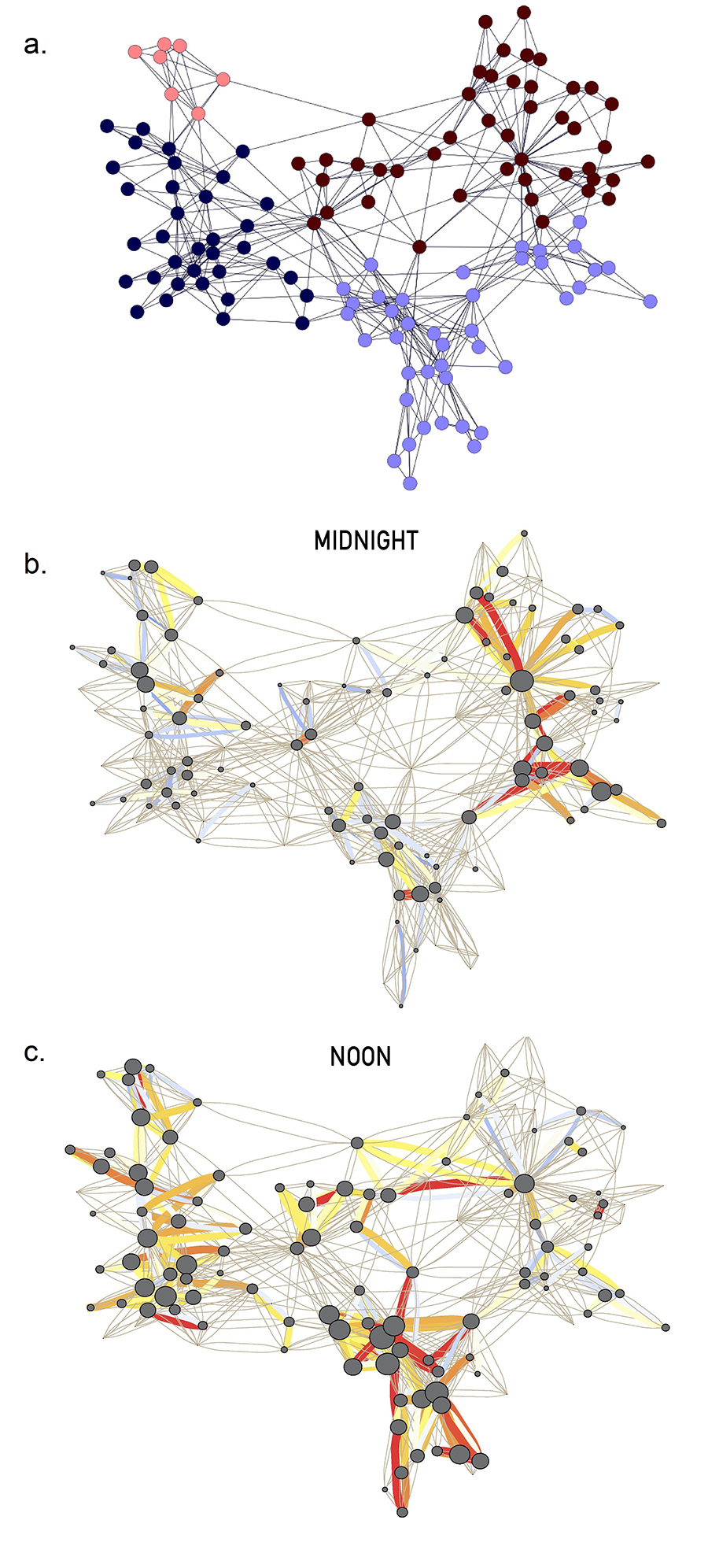
The answer was provided by Vincent Blondel and his students in 2007, who developed an algorithm to identify the country’s community structure. They started from the mobile call network, placing individuals next to whom they regularly called on their mobile phone [2]. The algorithm revealed that Belgium’s social network is broken into two large clusters of communities and that individuals in one of these clusters rarely talk with individuals from the other cluster (Image 9.1). The origin of this separation became obvious once they assigned to each node the language spoken by each individual, learning that one cluster consisted almost exclusively of French speakers and the other collected the Dutch speakers.
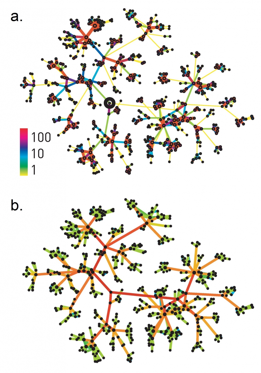
Image 9.1
Communities in Belgium
Communities extracted from the call pattern of the consumers of the largest Belgian mobile phone company. The network has about two million mobile phone users. The nodes correspond to communities, the size of each node being proportional to the number of individuals in the corresponding community. The color of each community on a red–green scale represents the language spoken in the particular community, red for French and green for Dutch. Only communities of more than 100 individuals are shown. The community that connects the two main clusters consists of several smaller communities with less obvious language separation, capturing the culturally mixed Brussels, the country’s capital. After [2].
In network science we call a community a group of nodes that have a higher likelihood of connecting to each other than to nodes from other communities. To gain intuition about community organization, next we discuss two areas where communities play a particularly important role:
Social Networks
Social networks are full of easy to spot communities, something that scholars have noticed decades ago [3,4,5,6,7]. Indeed, the employees of a company are more likely to interact with their coworkers than with employees of other companies [3]. Consequently work places appear as densely interconnected communities within the social network. Communities could also represent circles of friends, or a group of individuals who pursue the same hobby together, or individuals living in the same neighborhood.
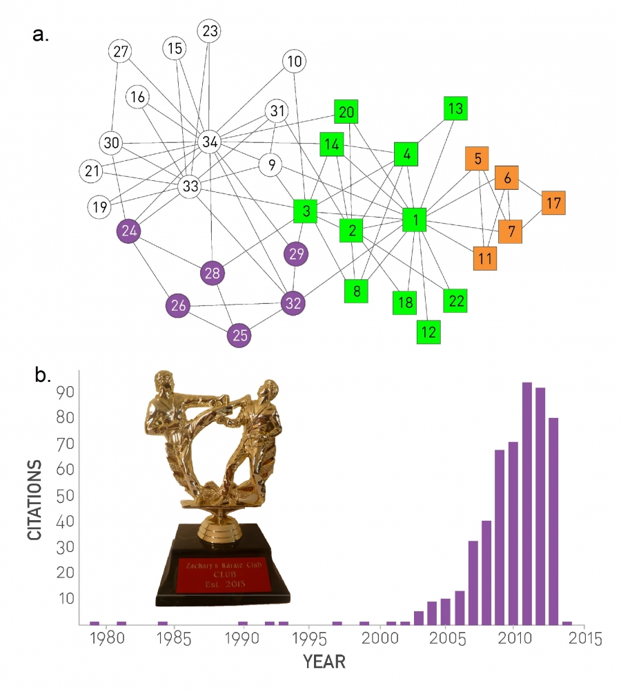
A social network that has received particular attention in the context of community detection is known as Zachary’s Karate Club (Image 9.2) [7], capturing the links between 34 members of a karate club. Given the club's small size, each club member knew everyone else. To uncover the true relationships between club members, sociologist Wayne Zachary documented 78 pairwise links between members who regularly interacted outside the club (Image 9.2a).
The interest in the dataset is driven by a singular event: A conflict between the club’s president and the instructor split the club into two. About half of the members followed the instructor and the other half the president, a breakup that unveiled the ground truth, representing club's underlying community structure (Image 9.2a). Today community finding algorithms are often tested based on their ability to infer these two communities from the structure of the network before the split.
Image 9.2
Zachary’s Karate Club
The connections between the 34 members of Zachary's Karate Club. Links capture interactions between the club members outside the club. The circles and the squares denote the two fractions that emerged after the club split in two. The colors capture the best community partition predicted by an algorithm that optimizes the modularity coefficient M (SECTION 9.4). The community boundaries closely follow the split: The white and purple communities capture one fraction and the green-orange communities the other. After [8].
The citation history of the Zachary karate club paper [7] mirrors the history of community detection in network science. Indeed, there was virtually no interest in Zachary’s paper until Girvan and Newman used it as a benchmark for community detection in 2002 [9]. Since then the number of citations to the paper exploded, reminiscent of the citation explosion to Erdős and Rényi’s work following the discovery of scale-free networks (Image 3.15).
The frequent use Zachary’s Karate Club network as a benchmark in community detection inspired the Zachary Karate Club Club, whose tongue-in-cheek statute states: “The first scientist at any conference on networks who uses Zachary's karate club as an example is inducted into the Zachary Karate Club Club, and awarded a prize.”
Hence the prize is not based on merit, but on the simple act of participation. Yet, its recipients are prominent network scientists (http://networkkarate.tumblr.com/). The figure shows the Zachary Karate Club trophy, which is always held by the latest inductee. Photo courtesy of Marián Boguñá.
Biological Networks
Communities play a particularly important role in our understanding of how specific biological functions are encoded in cellular networks. Two years before receiving the Nobel Prize in Medicine, Lee Hartwell argued that biology must move beyond its focus on single genes. It must explore instead how groups of molecules form functional modules to carry out a specific cellular functions [10]. Ravasz and collaborators [11] made the first attempt to systematically identify such modules in metabolic networks. They did so by building an algorithm to identify groups of molecules that form locally dense communities (Image 9.3).
Communities play a particularly important role in understanding human diseases. Indeed, proteins that are involved in the same disease tend to interact with each other [12,13]. This finding inspired the disease module hypothesis [14], stating that each disease can be linked to a well-defined neighborhood of the cellular network.
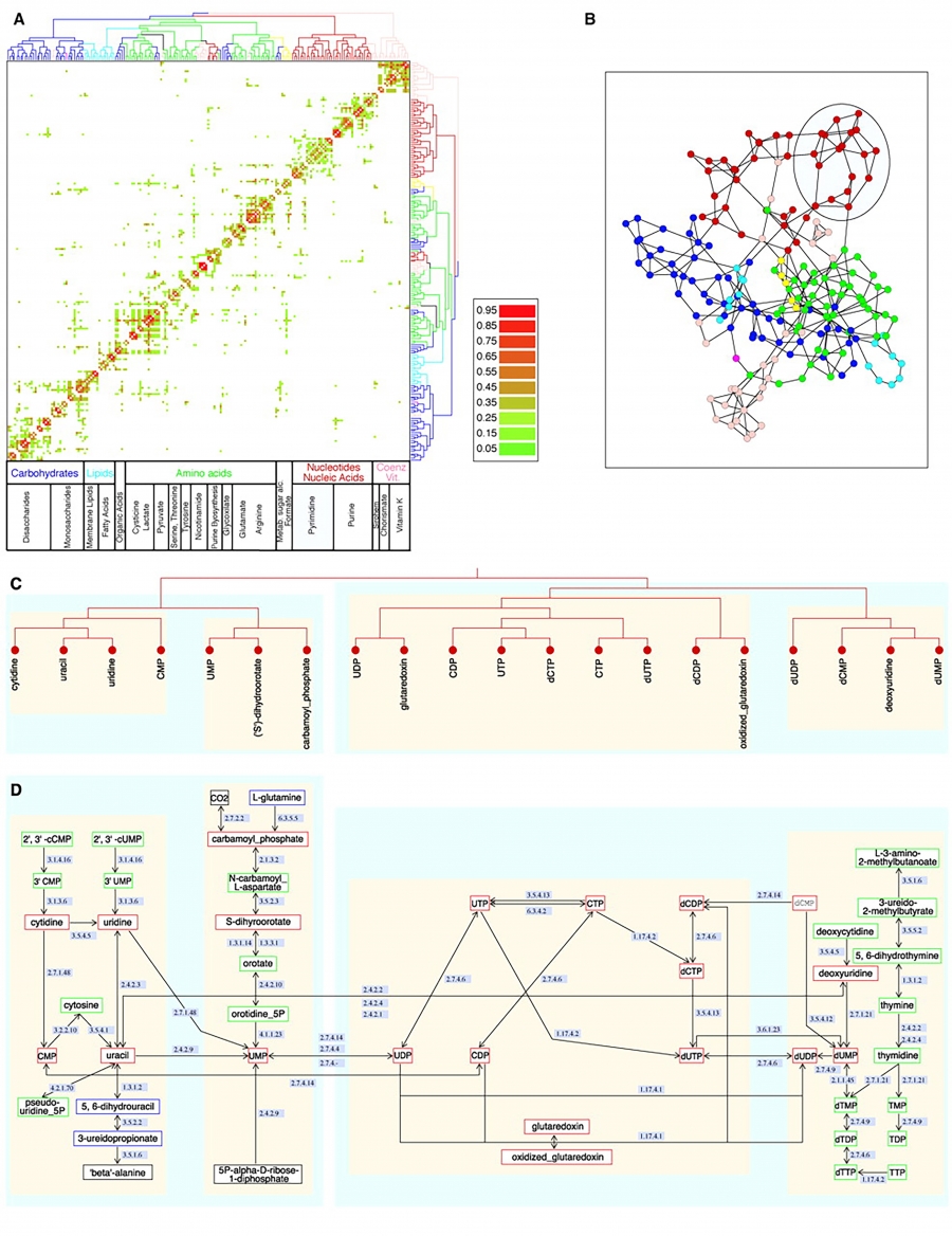
Image 9.3
Communities in Metabolic Networks
The E. coli metabolism offers a fertile ground to investigate the community structure of biological systems [11].
The biological modules (communities) identified by the Ravasz algorithm [11] (SECTION 9.3). The color of each node, capturing the predominant biochemical class to which it belongs, indicates that different functional classes are segregated in distinct network neighborhoods. The highlighted region selects the nodes that belong to the pyrimidine metabolism, one of the predicted communities.
The topologic overlap matrix of the E. coli metabolism and the corresponding dendrogram that allows us to identify the modules shown in (a). The color of the branches reflect the predominant biochemical role of the participating molecules, like carbohydrates (blue), nucleotide and nucleic acid metabolism (red), and lipid metabolism (cyan).
The red right branch of the dendrogram tree shown in (b), highlighting the region corresponding to the pyridine module.
The detailed metabolic reactions within the pyrimidine module. The boxes around the reactions highlight the communities predicted by the Ravasz algorithm.
After [11].
The examples discussed above illustrate the diverse motivations that drive community identification. The existence of communities is rooted in who connects to whom, hence they cannot be explained based on the degree distribution alone. To extract communities we must therefore inspect a network’s detailed wiring diagram. These examples inspire the starting hypothesis of this chapter:
H1: Fundamental Hypothesis
A network’s community structure is uniquely encoded in its wiring diagram.
According to the fundamental hypothesis there is a ground truth about a network’s community organization, that can be uncovered by inspecting Aij.
The purpose of this chapter is to introduce the concepts necessary to understand and identify the community structure of a complex network. We will ask how to define communities, explore the various community characteristics and introduce a series of algorithms, relying on different principles, for community identification.
Section 9.2
Basics of Communities
What do we really mean by a community? How many communities are in a network? How many different ways can we partition a network into communities? In this section we address these frequently emerging questions in community identification.
Defining Communities
Our sense of communities rests on a second hypothesis (Image 9.4):
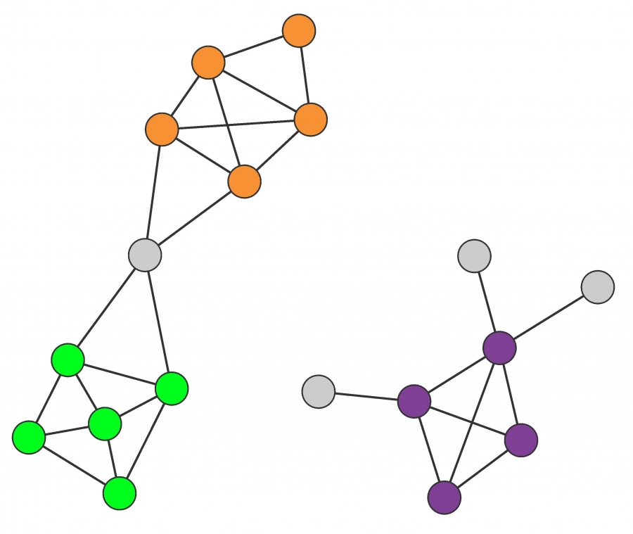
Image 9.4
Connectedness and Density Hypothesis
Communities are locally dense connected subgraphs in a network. This expectation relies on two distinct hypotheses:
Connectedness Hypothesis
Each community corresponds to a connected subgraph, like the subgraphs formed by the orange, green or the purple nodes. Consequently, if a network consists of two isolated components, each community is limited to only one component. The hypothesis also implies that on the same component a community cannot consist of two subgraphs that do not have a link to each other. Consequently, the orange and the green nodes form separate communities.
Density Hypothesis
Nodes in a community are more likely to connect to other members of the same community than to nodes in other communities. The orange, the green and the purple nodes satisfy this expectation.
After [11].
H2: Connectedness and Density Hypothesis
A community is a locally dense connected subgraph in a network.
In other words, all members of a community must be reached through other members of the same community (connectedness). At the same time we expect that nodes that belong to a community have a higher probability to link to the other members of that community than to nodes that do not belong to the same community (density). While this hypothesis considerably narrows what would be considered a community, it does not uniquely define it. Indeed, as we discuss below, several community definitions are consistent with H2.
Maximum Cliques
One of the first papers on community structure, published in 1949, defined a community as group of individuals whose members all know each other [5]. In graph theoretic terms this means that a community is a complete subgraph, or a clique. A clique automatically satisfies H2: it is a connected subgraph with maximal link density. Yet, viewing communities as cliques has several drawbacks:
While triangles are frequent in networks, larger cliques are rare.
Requiring a community to be a complete subgraph may be too restrictive, missing many other legitimate communities. For example, none of the communities of Image 9.2 and 9.3 correspond to complete subgraphs.
Strong and Weak Communities
To relax the rigidity of cliques, consider a connected subgraph C of NC nodes in a network. The internal degree kiint of node i is the number of links that connect i to other nodes in C. The external degree kiext is the number of links that connect i to the rest of the network. If kiext=0, each neighbor of i is within C, hence C is a good community for node i. If kiint=0, then node i should be assigned to a different community. These definitions allow us to distinguish two kinds of communities (Image 9.5):
Strong Community C is a strong community if each node within C has more links within the community than with the rest of the graph [15,16]. Specifically, a subgraph C forms a strong community if for each node i ∈ C,
Weak Community C is a weak community if the total internal degree of a subgraph exceeds its total external degree [16]. Specifically, a subgraph C forms a weak community if
A weak community relaxes the strong community requirement by allowing some nodes to violate (9.1). In other words, the inequality (9.2) applies to the community as a whole rather than to each node individually.
Note that each clique is a strong community, and each strong community is a weak community. The converse is generally not true (Image 9.5).
The community definitions discussed above (cliques, strong and weak communities) refine our notions of communities. At the same time they indicate that we do have some freedom in defining communities.
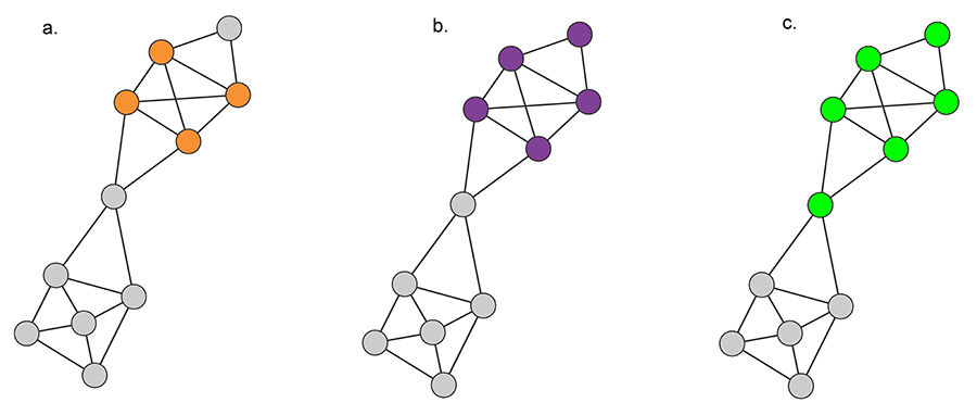
Image 9.5
Defining Communities
Cliques
A clique corresponds to a complete subgraph. The highest order clique of this network is a square, shown in orange. There are several three-node cliques on this network. Can you find them?
Strong Communities
A strong community, defined in (9.1), is a connected subgraph whose nodes have more links to other nodes in the same community that to nodes that belong to other communities. Such a strong community is shown in purple. There are additional strong communities on the graph - can you find at least two more?
Weak Communities
A weak community defined in (9.2) is a subgraph whose nodes’ total internal degree exceeds their total external degree. The green nodes represent one of the several possible weak communities of this network.
Number of Communities
How many ways can we group the nodes of a network into communities? To answer this question consider the simplest community finding problem, called graph bisection: We aim to divide a network into two non-overlapping subgraphs, such that the number of links between the nodes in the two groups, called the cut size, is minimized (BOX 9.1).
Graph Partitioning
We can solve the graph bisection problem by inspecting all possible divisions into two groups and choosing the one with the smallest cut size. To determine the computational cost of this brute force approach we note that the number of distinct ways we can partition a network of N nodes into groups of N1 and N2 nodes is
Using Stirling's formula
we can write (9.3) as
To simplify the problem let us set the goal of dividing the network into two equal sizes N1 = N2 = N/2. In this case (9.4) becomes
indicating that the number of bisections increases exponentially with the size of the network.
To illustrate the implications of (9.5) consider a network with ten nodes which we bisect into two subgraphs of size N1 = N2 = 5. According to (9.3) we need to check 252 bisections to find the one with the smallest cut size. Let us assume that our computer can inspect these 252 bisections in one millisecond (10-3 sec). If we next wish to bisect a network with a hundred nodes into groups with N1 = N2 = 50, according to (9.3) we need to check approximately 1029 divisions, requiring about 1016 years on the same computer. Therefore our brute-force strategy is bound to fail, being impossible to inspect all bisections for even a modest size network.
Community Detection
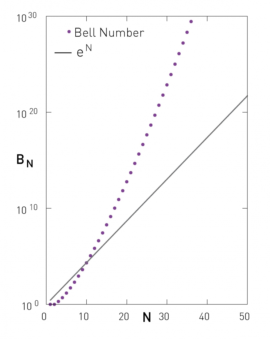
While in graph partitioning the number and the size of communities is predefined, in community detection both parameters are unknown. We call a partition a division of a network into an arbitrary number of groups, such that each node belongs to one and only one group. The number of possible partitions follows [19-22]
As Image 9.7 indicates, BN grows faster than exponentially with the network size for large N.
Equations (9.5) and (9.6) signal the fundamental challenge of community identification: The number of possible ways we can partition a network into communities grows exponentially or faster with the network size N. Therefore it is impossible to inspect all partitions of a large network (BOX 9.2).
Image 9.7
Number of Partitions
The number of partitions of a network of size N is provided by the Bell number (9.6). The figure compares the Bell number to an exponential function, illustrating that the number of possible partitions grows faster than exponentially. Given that there are over 1040 partitions for a network of size N=50, brute-force approaches that aim to identify communities by inspecting all possible partitions are computationally infeasible.
In summary, our notion of communities rests on the expectation that each community corresponds to a locally dense connected subgraph. This hypothesis leaves room for numerous community definitions, from cliques to weak and strong communities. Once we adopt a definition, we could identify communities by inspecting all possible partitions of a network, selecting the one that best satisfies our definition. Yet, the number of partitions grows faster than exponentially with the network size, making such brute-force approaches computationally infeasible. We therefore need algorithms that can identify communities without inspecting all partitions. This is the subject of the next sections.
Section 9.3
Hierarchical Clustering
To uncover the community structure of large real networks we need algorithms whose running time grows polynomially with N. Hierarchical clustering, the topic of this section, helps us achieve this goal.
The starting point of hierarchical clustering is a similarity matrix, whose elements xij indicate the distance of node i from node j. In community identification the similarity is extracted from the relative position of nodes i and j within the network.
Once we have xij, hierarchical clustering iteratively identifies groups of nodes with high similarity. We can use two different procedures to achieve this: agglomerative algorithms merge nodes with high similarity into the same community, while divisive algorithms isolate communities by removing low similarity links that tend to connect communities. Both procedures generate a hierarchical tree, called a dendrogram, that predicts the possible community partitions. Next we explore the use of agglomerative and divisive algorithms to identify communities in networks.
Agglomerative Procedures: the Ravasz Algorithm
We illustrate the use of agglomerative hierarchical clustering for community detection by discussing the Ravasz algorithm, proposed to identify functional modules in metabolic networks [11]. The algorithm consists of the following steps:
Step 1: Define the Similarity Matrix
In an agglomerative algorithm similarity should be high for node pairs that belong to the same community and low for node pairs that belong to different communities. In a network context nodes that connect to each other and share neighbors likely belong to the same community, hence their xij should be large. The topological overlap matrix (Image 9.9) [11]
captures this expectation. Here Θ(x) is the Heaviside step function, which is zero for x≤0 and one for x>0; J(i, j) is the number of common neighbors of node i and j, to which we add one (+1) if there is a direct link between i and j; min(ki,kj) is the smaller of the degrees ki and kj. Consequently:
xij0=1 if nodes i and j have a link to each other and have the same neighbors, like A and B in Image 9.9a.
xij0(i, j) =0 if i and j do not have common neighbors, nor do they link to each other, like A and E.
Members of the same dense local network neighborhood have high topological overlap, like nodes H, I, J, K or E, F, G.
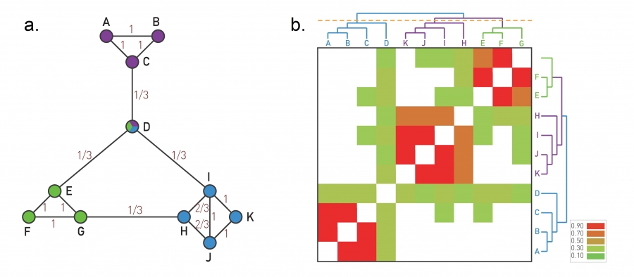
Image 9.9
The Ravasz Algorithm
The agglomerative hierarchical clustering algorithm proposed by Ravasz was designed to identify functional modules in metabolic networks, but it can be applied to arbitrary networks.
Topological Overlap
A small network illustrating the calculation of the topological overlap xij0. For each node pair i and j we calculate the overlap (9.7). The obtained xij0 for each connected node pair is shown on each link. Note that xij0 can be nonzero for nodes that do not link to each other, but have a common neighbor. For example, xij=1/3 for C and E.
Topological Overlap Matrix
The topological overlap matrix xij0 for the network shown in (a). The rows and columns of the matrix were reordered after applying average linkage clustering, placing next to each other nodes with the highest topological overlap. The colors denote the degree of topological overlap between each node pair, as calculated in (a). By cutting the dendrogram with the orange line, it recovers the three modules built into the network. The dendogram indicates that the EFG and the HIJK modules are closer to each other than they are to the ABC module.
After [11].
Step 2: Decide Group Similarity
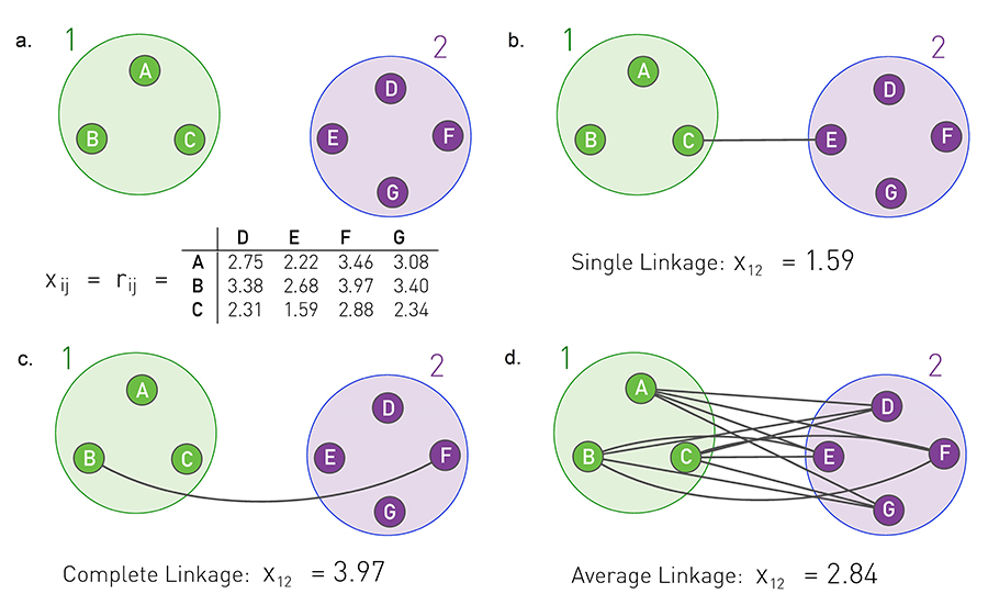
As nodes are merged into small communities, we must measure how similar two communities are. Three approaches, called single, complete and average cluster similarity, are frequently used to calculate the community similarity from the node-similarity matrix xij (Image 9.10). The Ravasz algorithm uses the average cluster similarity method, defining the similarity of two communities as the average of xij over all node pairs i and j that belong to distinct communities (Image 9.10d).
Image 9.10
Cluster Similarity
In agglomerative clustering we need to determine the similarity of two communities from the node similarity matrix xij . We illustrate this procedure for a set of points whose similarity xij is the physical distance rij between them. In networks xij corresponds to some network-based distance measure, like xij o defined in (9.7).
Similarity Matrix
Seven nodes forming two distinct communities. The table shows the distance rij between each node pair, acting as the similarity xij.
Single Linkage Clustering
The similarity between communities 1 and 2 is the smallest of all xij , where i and j are in different communities. Hence the similarity is x12=1.59, corresponding to the distance between nodes C and E.
Complete Linkage Clustering
The similarity between two communities is the maximum of xij , where i and j are in distinct communities. Hence x12=3.97.
Average Linkage Clustering
The similarity between two communities is the average of xij over all node pairs i and j that belong to different communities. This is the procedure implemented in the Ravasz algorithm, providing x12=2.84.
Step 3: Apply Hierarchical Clustering
The Ravasz algorithm uses the following procedure to identify the communities:
Assign each node to a community of its own and evaluate xij for all node pairs.
Find the community pair or the node pair with the highest similarity and merge them into a single community.
Calculate the similarity between the new community and all other communities.
Repeat Steps 2 and 3 until all nodes form a single community.
Step 4: Dendrogram
The pairwise mergers of Step 3 will eventually pull all nodes into a single community. We can use a dendrogram to extract the underlying community organization.
The dendrogram visualizes the order in which the nodes are assigned to specific communities. For example, the dendrogram of Image 9.9b tells us that the algorithm first merged nodes A with B, K with J and E with F, as each of these pairs have xij0=1. Next node C was added to the (A, B) community, I to (K, J) and G to (E, F).
To identify the communities we must cut the dendrogram. Hierarchical clustering does not tell us where that cut should be. Using for example the cut indicated as a dashed line in Image 9.9b, we recover the three obvious communities (ABC, EFG, and HIJK).
Applied to the E. coli metabolic network (Image 9.3a), the Ravasz algorithm identifies the nested community structure of bacterial metabolism. To check the biological relevance of these communities, we color-coded the branches of the dendrogram according to the known biochemical classification of each metabolite. As shown in Image 9.3b, substrates with similar biochemical role tend to be located on the same branch of the tree. In other words the known biochemical classification of these metabolites confirms the biological relevance of the communities extracted from the network topology.
Computational Complexity
How many computations do we need to run the Ravasz algorithm? The algorithm has four steps, each with its own computational complexity:
Step 1:
The calculation of the similarity matrix xij0 requires us to compare N2 node pairs, hence the number of computations scale as N2. In other words its computational complexity is 0(N2).
Step 2:
Group similarity requires us to determine in each step the distance of the new cluster to all other clusters. Doing this N times requires 0(N2) calculations.
Steps 3 & 4:
The construction of the dendrogram can be performed in 0(NlogN) steps.
Combining Steps 1-4, we find that the number of required computations scales as 0(N2) + 0(N2) + 0(NlogN). As the slowest step scales as 0(N2), the algorithm’s computational complexity is 0(N2). Hence hierarchal clustering is much faster than the brute force approach, which generally scales as 0(eN).
Divisive Procedures: the Girvan-Newman Algorithm
Divisive procedures systematically remove the links connecting nodes that belong to different communities, eventually breaking a network into isolated communities. We illustrate their use by introducing an algorithm proposed by Michelle Girvan and Mark Newman [9,23], consisting of the following steps:
Step 1: Define Centrality
While in agglomerative algorithms xij selects node pairs that belong to the same community, in divisive algorithms xij, called centrality, selects node pairs that are in different communities. Hence we want xij to be high (or low) if nodes i and j belong to different communities and small if they are in the same community. Three centrality measures that satisfy this expectation are discussed in Image 9.11. The fastest of the three is link betweenness, defining xij as the number of shortest paths that go through the link (i, j). Links connecting different communities are expected to have large xij while links within a community have small xij.
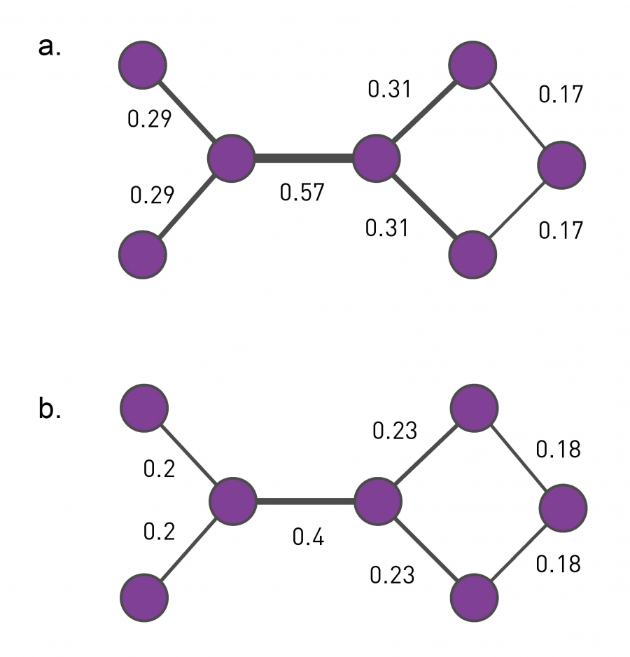
Image 9.11
Centrality Measures
Divisive algorithms require a centrality measure that is high for nodes that belong to different communities and is low for node pairs in the same community. Two frequently used measures can achieve this:
Link Betweenness
Link betweenness captures the role of each link in information transfer. Hence xij is proportional to the number of shortest paths between all node pairs that run along the link (i,j). Consequently, inter-community links, like the central link in the figure with xij =0.57, have large betweenness. The calculation of link betweenness scales as 0(LN), or 0(N2) for a sparse network [23].
Random-Walk Betweenness
A pair of nodes m and n are chosen at random. A walker starts at m, following each adjacent link with equal probability until it reaches n. Random walk betweenness xij is the probability that the link i→j was crossed by the walker after averaging over all possible choices for the starting nodes m and n. The calculation requires the inversion of an NxN matrix, with 0(N3) computational complexity and averaging the flows over all node pairs, with 0(LN2). Hence the total computational complexity of random walk betweenness is 0[(L + N) N2], or 0(N3) for a sparse network.
Step 2: Hierarchical Clustering
The final steps of a divisive algorithm mirror those we used in agglomerative clustering (Image 9.12):
Compute the centrality xij of each link.
Remove the link with the largest centrality. In case of a tie, choose one link randomly.
Recalculate the centrality of each link for the altered network.
Repeat steps 2 and 3 until all links are removed.
Girvan and Newman applied their algorithm to Zachary’s Karate Club (Image 9.2a), finding that the predicted communities matched almost perfectly the two groups after the break-up. Only node 3 was classified incorrectly.
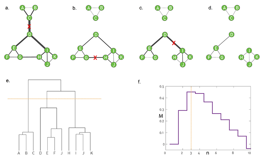
Image 9.12
The Girvan-Newman Algorithm
Divisive algorithms require a centrality measure that is high for nodes that belong to different communities and is low for node pairs in the same community. Two frequently used measures can achieve this:
(a) The divisive hierarchical algorithm of Girvan and Newman uses link betweenness (Image 9.11a) as centrality. In the figure the link weights, assigned proportionally to xij, indicate that links connecting different communities have the highest xij. Indeed, each shortest path between these communities must run through them.
(b)-(d) The sequence of images illustrates how the algorithm removes one-by-one the three highest xij links, leaving three isolated communities behind. Note that betweenness needs to be recalculated after each link removal.
(e) The dendrogram generated by the Girvan-Newman algorithm. The cut at level 3, shown as an orange dotted line, reproduces the three communities present in the network.
(f) The modularity function, M, introduced in SECTION 9.4, helps us select the optimal cut. Its maxima agrees with our expectation that the best cut is at level 3, as shown in (e).
Computational Complexity
The rate limiting step of divisive algorithms is the calculation of centrality. Consequently the algorithm’s computational complexity depends on which centrality measure we use. The most efficient is link betweenness, with 0(LN) [24,25,26] (Image 9.11a). Step 3 of the algorithm introduces an additional factor L in the running time, hence the algorithm scales as 0(L2N), or 0(N3) for a sparse network.
Hierarchy in Real Networks
Hierarchical clustering raises two fundamental questions:
Nested Communities
First, it assumes that small modules are nested into larger ones. These nested communities are well captured by the dendrogram (Image 9.9b and 9.12e). How do we know, however, if such hierarchy is indeed present in a network? Could this hierarchy be imposed by our algorithms, whether or not the underlying network has a nested community structure? Communities and the Scale-Free Property Second, the density hypothesis states that a network can be partitioned into a collection of subgraphs that are only weakly linked to other subgraphs. How can we have isolated communities in a scale-free network, if the hubs inevitably link multiple communities?
The hierarchical network model, whose construction is shown in Image 9.13, resolves the conflict between communities and the scale-free property and offers intuition about the structure of nested hierarchical communities. The obtained network has several key characteristics:
Scale-free Property
The hierarchical model generates a scale-free network with degree exponent (Image 9.14a, ADVANCED TOPICS 9.A)
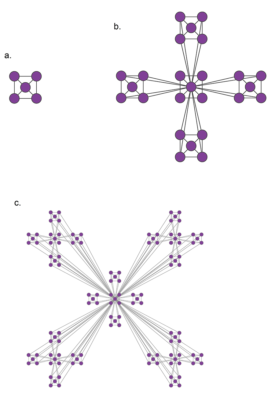
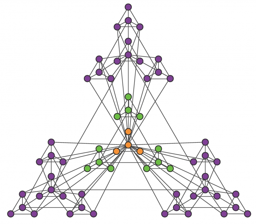
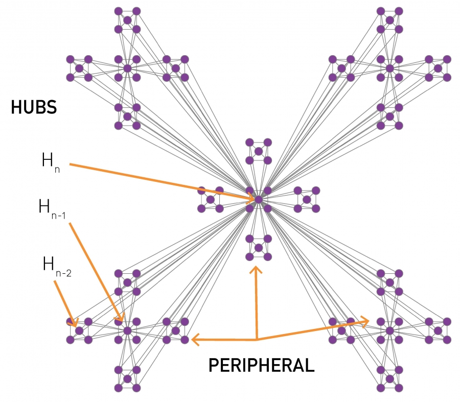
Image 9.13
Hierarchical Network
The iterative construction of a deterministic hierarchical network.
Start from a fully connected module of five nodes. Note that the diagonal nodes are also connected, but the links are not visible.
Create four identical replicas of the starting module and connect the peripheral nodes of each module to the central node of the original module. This way we obtain a network with N=25 nodes.
Create four replicas of the 25-node module and connect the peripheral nodes again to the central node of the original module, obtaining an N=125-node network. This process is continued indefinitely.
After [27].
Size Independent Clustering Coefficient
While for the Erdős-Rényi and the Barabási-Albert models the clustering coefficient decreases with N (SECTION 5.9), for the hierarchical network we have C=0.743 independent of the network size (Image 9.14c). Such N-independent clustering coefficient has been observed in metabolic networks [11].
Hierarchical Modularity
The model consists of numerous small communities that form larger communities, which again combine into ever larger communities. The quantitative signature of this nested hierarchical modularity is the dependence of a node’s clustering coefficient on the node’s degree [11,27,28]
In other words, the higher a node’s degree, the smaller is its clustering coefficient.
Equation (9.8) captures the way the communities are organized in a network. Indeed, small degree nodes have high C because they reside in dense communities. High degree nodes have small C because they connect to different communities. For example, in Image 9.13c the nodes at the center of the five-node modules have k=4 and clustering coefficient C=4. Those at the center of a 25-node module have k=20 and C=3/19. Those at the center of the 125-node modules have k=84 and C=3/83. Hence the higher the degree of a node, the smaller is its C.
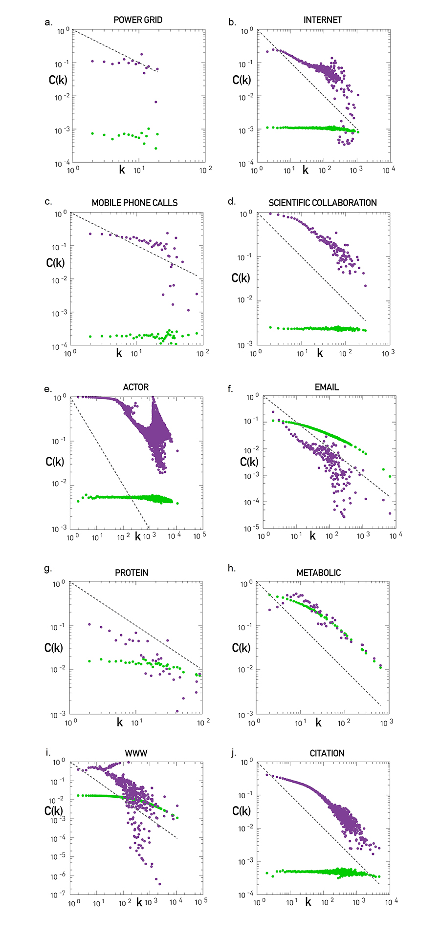
The hierarchical network model suggests that inspecting C(k) allows us to decide if a network is hierarchical. For the Erdős-Rényi and the Barabási-Albert models C(k) is independent of k, indicating that they do not display hierarchical modularity. To see if hierarchical modularity is present in real systems, we calculated C(k) for ten reference networks, finding that (Image 9.36):
Only the power grid lacks hierarchical modularity, its C(k) being independent of k (Image 9.36a).
For the remaining nine networks C(k) decreases with k. Hence in these networks small nodes are part of small dense communities, while hubs link disparate communities to each other.
For the scientific collaboration, metabolic, and citation network C(k) follows (9.8) in the high-k region. The form of C(k) for the Internet, mobile, email, protein interactions, and the WWW needs to be derived individually, as for those C(k) does not follow (9.8). More detailed network models predict C(k)~k-β, where β is between 0 and 2 [27,28].
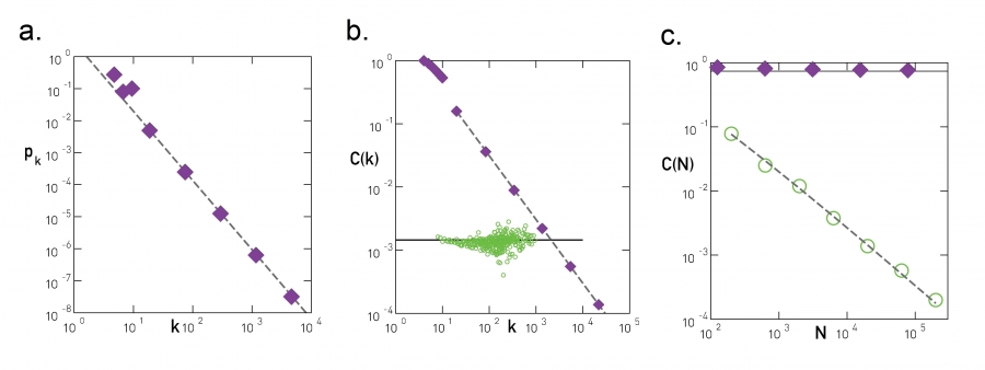
Image 9.14
Scaling in Hierarchical Networks
Three quantities characterize the hierarchical network shown in Image 9.13:
Degree Distribution
The scale-free nature of the generated network is illustrated by the scaling of pk with slope γ=ln 5/ln 4, shown as a dashed line. See ADVANCED TOPICS 9.A for the derivation of the degree exponent.
Hierarchical Clustering C(k) follows (9.8), shown as a dashed line. The circles show C(k) for a randomly wired scale-free network, obtained from the original model by degree-preserving randomization. The lack of scaling indicates that the hierarchical architecture is lost under rewiring. Hence C(k) captures a property that goes beyond the degree distribution.
Size Independent Clustering Coefficient
The dependence of the clustering coefficient C on the network size N. For the hierarchical model C is independent of N (filled symbols), while for the Barabási-Albert model C(N) decreases (empty symbols).
After [27].
In summary, in principle hierarchical clustering does not require preliminary knowledge about the number and the size of communities. In practice it generates a dendrogram that offers a family of community partitions characterizing the studied network. This dendrogram does not tell us which partition captures best the underlying community structure. Indeed, any cut of the hierarchical tree offers a potentially valid partition (Image 9.15). This is at odds with our expectation that in each network there is a ground truth, corresponding to a unique community structure.
While there are multiple notions of hierarchy in networks [29,30], inspecting C(k) helps decide if the underlying network has hierarchical modularity. We find that C(k) decreases in most real networks, indicating that most real systems display hierarchical modularity. At the same time C(k) is independent of k for the Erdős-Rényi or Barabási-Albert models, indicating that these canonical models lack a hierarchical organization.
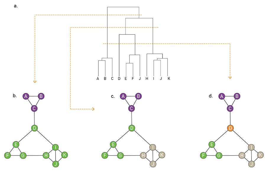
Image 9.15
Ambiguity in Hierarchical Clustering
Hierarchical clustering does not tell us where to cut a dendrogram. Indeed, depending on where we make the cut in the dendrogram of Image 9.9a, we obtain (b) two, (c) three or (d) four communities. While for a small network we can visually decide which cut captures best the underlying community structure, it is impossible to do so in larger networks. In the next section we discuss modularity, that helps us select the optimal cut.
Section 9.4
Modularity
In a randomly wired network the connection pattern between the nodes is expected to be uniform, independent of the network's degree distribution. Consequently these networks are not expected to display systematic local density fluctuations that we could interpret as communities. This expectation inspired the third hypothesis of community organization:
H3: Random Hypothesis
Randomly wired networks lack an inherent community structure.
This hypothesis has some actionable consequences: By comparing the link density of a community with the link density obtained for the same group of nodes for a randomly rewired network, we could decide if the original community corresponds to a dense subgraph, or its connectivity pattern emerged by chance.
In this section we show that systematic deviations from a random configuration allow us to define a quantity called modularity, that measures the quality of each partition. Hence modularity allows us to decide if a particular community partition is better than some other one. Finally, modularity optimization offers a novel approach to community detection.
Modularity
Consider a network with N nodes and L links and a partition into nc communities, each community having Nc nodes connected to each other by Lc links, where c=1,...,nc. If Lc is larger than the expected number of links between the Nc nodes given the network’s degree sequence, then the nodes of the subgraph Cc could indeed be part of a true community, as expected based on the Density Hypothesis H2 (Image 9.2). We therefore measure the difference between the network’s real wiring diagram (Aij) and the expected number of links between i and j if the network is randomly wired (pij),
Here pij can be determined by randomizing the original network, while keeping the expected degree of each node unchanged. Using the degree preserving null model (7.1) we have
If Mc is positive, then the subgraph Cc has more links than expected by chance, hence it represents a potential community. If Mc is zero then the connectivity between the Nc nodes is random, fully explained by the degree distribution. Finally, if Mc is negative, then the nodes of Cc do not form a community.
Using (9.10) we can derive a simpler form for the modularity (9.9) (ADVANCED TOPICS 9.B)
where Lc is the total number of links within the community Cc and kc is the total degree of the nodes in this community.
To generalize these ideas to a full network consider the complete partition that breaks the network into nc communities. To see if the local link density of the subgraphs defined by this partition differs from the expected density in a randomly wired network, we define the partition’s modularity by summing (9.11) over all nc communities [23]
Modularity has several key properties:
Higher Modularity Implies Better Partition
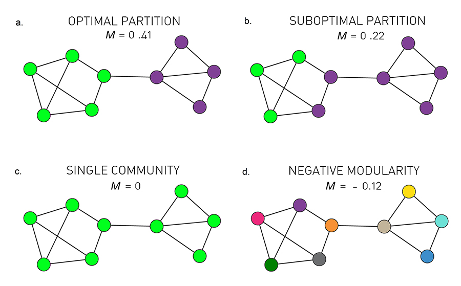
The higher is M for a partition, the better is the corresponding community structure. Indeed, in Image 9.16a the partition with the maximum modularity (M=0.41) accurately captures the two obvious communities. A partition with a lower modularity clearly deviates from these communities (Image 9.16b). Note that the modularity of a partition cannot exceed one [31,32].
Zero and Negative Modularity
By taking the whole network as a single community we obtain M=0, as in this case the two terms in the parenthesis of (9.12) are equal (Image 9.16c). If each node belongs to a separate community, we have Lc=0 and the sum (9.12) has nc negative terms, hence M is negative (Image 9.16d).
Image 9.16
Modularity
To better understand the meaning of modularity, we show M defined in (9.12) for several partitions of a network with two obvious communities.
Optimal Partition
The partition with maximal modularity M=0.41 closely matches the two distinct communities.
Suboptimal Partition
A partition with a sub-optimal but positive modularity, M=0.22, fails to correctly identify the communities present in the network.
Single Community
If we assign all nodes to the same community we obtain M=0, independent of the network structure.
Negative Modularity
If we assign each node to a different community, modularity is negative, obtaining M=-0.12.
We can use modularity to decide which of the many partitions predicted by a hierarchical method offers the best community structure, selecting the one for which M is maximal. This is illustrated in Image 9.12f, which shows M for each cut of the dendrogram, finding a clear maximum when the network breaks into three communities.
The Greedy Algorithm
The expectation that partitions with higher modularity corresponds to partitions that more accurately capture the underlying community structure prompts us to formulate our final hypothesis:
H4: Maximal Modularity Hypothesis
For a given network the partition with maximum modularity corresponds to the optimal community structure.
The hypothesis is supported by the inspection of small networks, for which the maximum M agrees with the expected communities (Image 9.12 and 9.16).
The maximum modularity hypothesis is the starting point of several community detection algorithms, each seeking the partition with the largest modularity. In principle we could identify the best partition by checking M for all possible partitions, selecting the one for which M is largest. Given, however, the exceptionally large number of partitions, this bruteforce approach is computationally not feasible. Next we discuss an algorithm that finds partitions with close to maximal M, while bypassing the need to inspect all partitions.
Greedy Algorithm
The first modularity maximization algorithm, proposed by Newman [33], iteratively joins pairs of communities if the move increases the partition's modularity. The algorithm follows these steps:
Assign each node to a community of its own, starting with N communities of single nodes.
Inspect each community pair connected by at least one link and compute the modularity difference ΔM obtained if we merge them. Identify the community pair for which ΔM is the largest and merge them. Note that modularity is always calculated for the full network.
Repeat Step 2 until all nodes merge into a single community, recording M for each step.
Select the partition for which M is maximal.
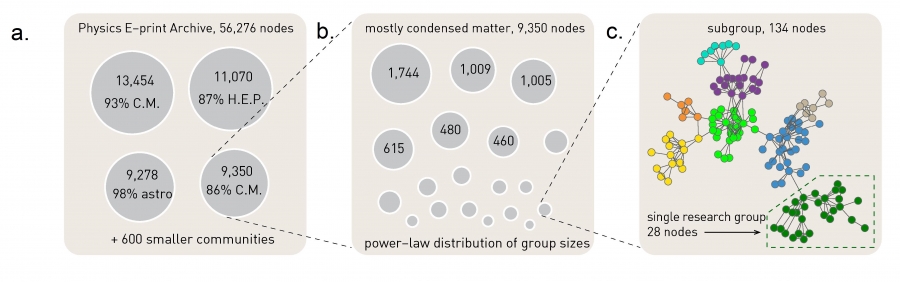
To illustrate the predictive power of the greedy algorithm consider the collaboration network between physicists, consisting of N=56,276 scientists in all branches of physics who posted papers on arxiv.org (Image 9.17). The greedy algorithm predicts about 600 communities with peak modularity M = 0.713. Four of these communities are very large, together containing 77% of all nodes (Image 9.17a). In the largest community 93% of the authors publish in condensed matter physics while 87% of the authors in the second largest community publish in high energy physics, indicating that each community contains physicists of similar professional interests. The accuracy of the greedy algorithm is also illustrated in Image 9.2a, showing that the community structure with the highest M for the Zachary Karate Club accurately captures the club’s subsequent split.
Image 9.17
The Greedy Algorithm
Clustering Physicists
The community structure of the collaboration network of physicists. The greedy algorithm predicts four large communities, each composed primarily of physicists of similar interest. To see this on each cluster we show the percentage of members who belong to the same subfield of physics. Specialties are determined by the subsection(s) of the e-print archive in which individuals post papers. C.M. indicates condensed matter, H.E.P. high-energy physics, and astro astrophysics. These four large communities coexist with 600 smaller communities, resulting in an overall modularity M=0.713.
Identifying Subcommunities
We can identify subcommunities by applying the greedy algorithm to each community, treating them as separate networks. This procedure splits the condensed matter community into many smaller subcommunities, increasing the modularity of the partition to M=0.807.
Research Groups
One of these smaller communities is further partitioned, revealing individual researchers and the research groups they belong to.
After [33].
Computational Complexity
Since the calculation of each ΔM can be done in constant time, Step 2 of the greedy algorithm requires O(L) computations. After deciding which communities to merge, the update of the matrix can be done in a worstcase time O(N). Since the algorithm requires N–1 community mergers, its complexity is O[(L + N)N], or O(N2) on a sparse graph. Optimized implementations reduce the algorithm’s complexity to O(Nlog2N) (Online Resource 9.1).
Limits of Modularity
Given the important role modularity plays in community identification, we must be aware of some of its limitations.
Resolution Limit
Modularity maximization forces small communities into larger ones [34]. Indeed, if we merge communities A and B into a single community, the network’s modularity changes with (ADVANCED TOPICS 9.B)
where lAB is number of links that connect the nodes in community A with total degree kA to the nodes in community B with total degree kB. If A and B are distinct communities, they should remain distinct when M is maximized. As we show next, this is not always the case.
Consider the case when kAkB|2L < 1, in which case (9.13) predicts ΔMAB > 0 if there is at least one link between the two communities (lAB ≥ 1). Hence we must merge A and B to maximize modularity. Assuming for simplicity that kA ~ kB= k, if the total degree of the communities satisfies
then modularity increases by merging A and B into a single community, even if A and B are otherwise distinct communities. This is an artifact of modularity maximization: if kA and kB are under the threshold (9.14), the expected number of links between them is smaller than one. Hence even a single link between them will force the two communities together when we maximize M. This resolution limit has several consequences:
Modularity maximization cannot detect communities that are smaller than the resolution limit (9.14). For example, for the WWW sample with L=1,497,134 (Table 2.1) modularity maximization will have difficulties resolving communities with total degree kC ≲ 1,730.
Real networks contain numerous small communities [36-38]. Given the resolution limit (9.14), these small communities are systematically forced into larger communities, offering a misleading characterization of the underlying community structure.
There are several widely used community finding algorithms that maximize modularity.
Optimized Greedy Algorithm The use of data structures for sparse matrices can decrease the greedy algorithm’s computational complexity to 0(Nlog2N) [35]. See http://cs.unm.edu/~aaron/research/fastmodularity. htm for the code.
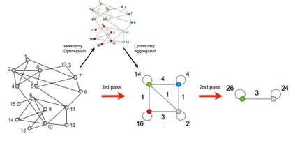
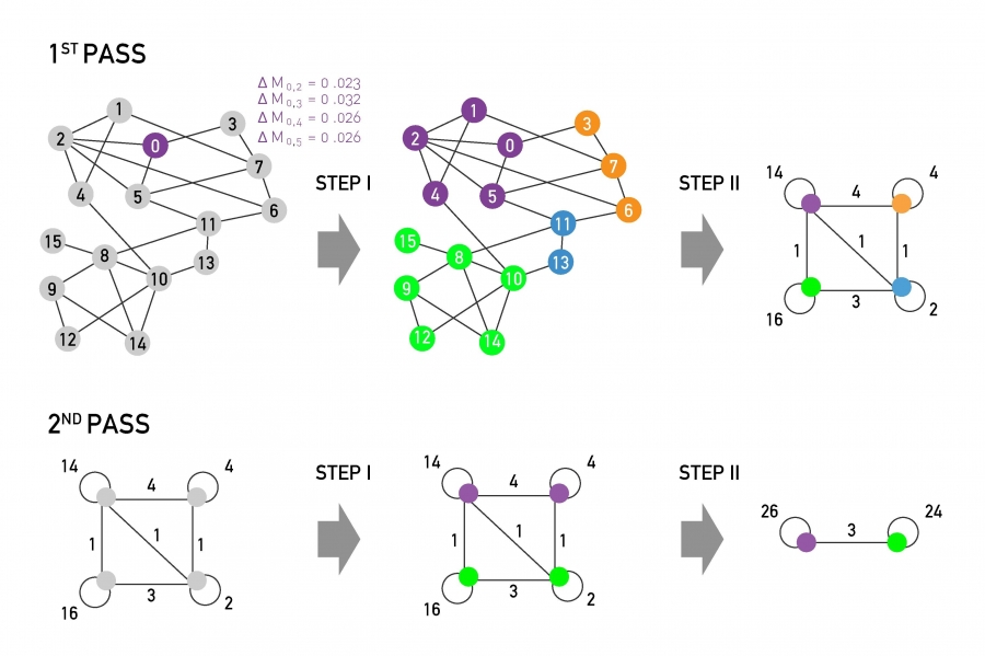
Louvain Algorithm The modularity optimization algorithm achieves a computational complexity of 0(L) [2]. Hence it allows us to identify communities in networks with millions of nodes, as illustrated in Figure 9.1. The algorithm is described in ADVANCED TOPICS 9.C. See https:// sites.google.com/site/findcommunities/ for the code
To avoid the resolution limit we can further subdivide the large communities obtained by modularity optimization [33,34,39]. For example, treating the smaller of the two condensed-matter groups of Image 9.17a as a separate network and feeding it again into the greedy algorithm, we obtain about 100 smaller communities with an increased modularity M = 0.807 (Image 9.17b) [33].
Modularity Maxima
All algorithms based on maximal modularity rely on the assumption that a network with a clear community structure has an optimal partition with a maximal M [40]. In practice we hope that Mmax is an easy to find maxima and that the communities predicted by all other partitions are distinguishable from those corresponding to Mmax. Yet, as we show next, this optimal partition is difficult to identify among a large number of close to optimal partitions.
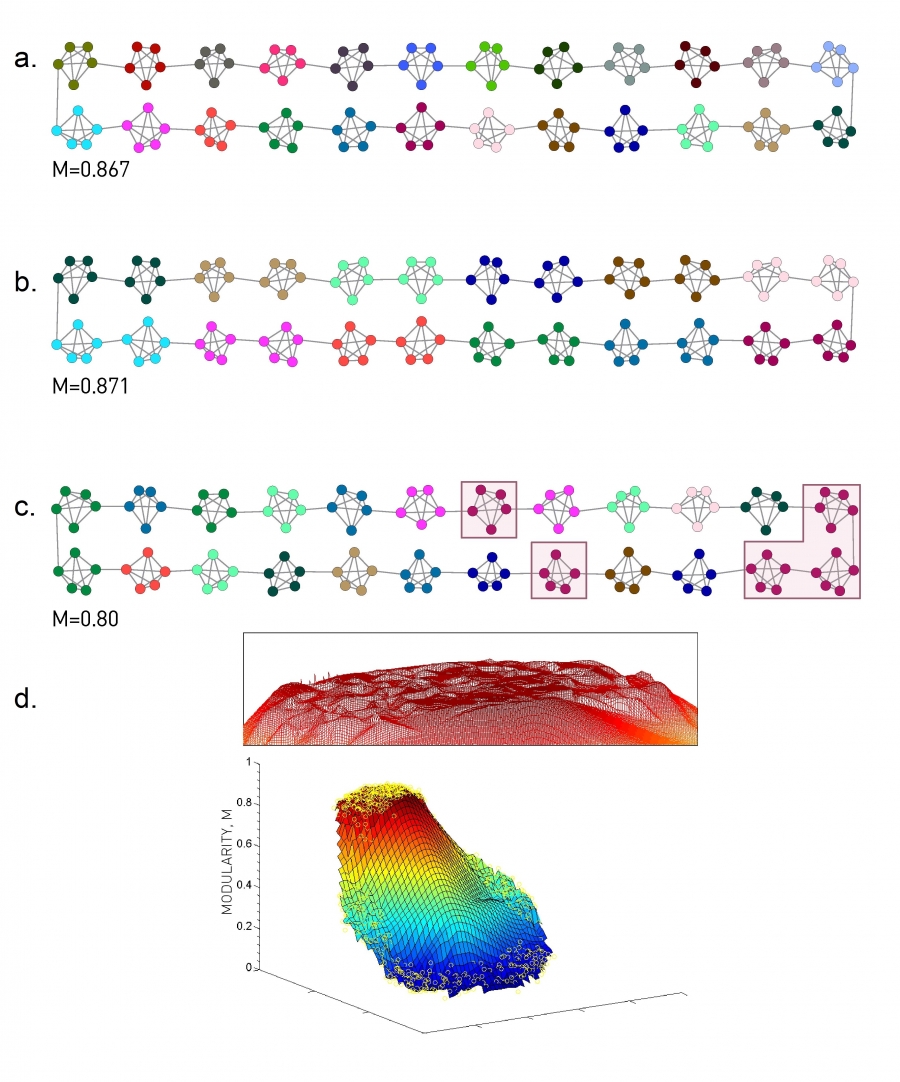
Consider a network composed of nc subgraphs with comparable link densities kC ≈ 2L/nc. The best partition should correspond to the one where each cluster is a separate community (Image 9.18a), in which case M=0.867. Yet, if we merge the neighboring cluster pairs into a single community we obtain a higher modularity M=0.87 (Image 9.18b). In general (9.13) and (9.14) predicts that if we merge a pair of clusters, we change modularity with
In other words the drop in modularity is less than ΔM = −2/nc2. For a network with nc = 20 communities, this change is at most ΔM = −0.005, tiny compared to the maximal modularity M≃0.87 (Image 9.18b). As the number of groups increases, ΔMij goes to zero, hence it becomes increasingly difficult to distinguish the optimal partition from the numerous suboptimal alternatives whose modularity is practically indistinguishable from Mmax. In other words, the modularity function is not peaked around a single optimal partition, but has a high modularity plateau (Image 9.18d).
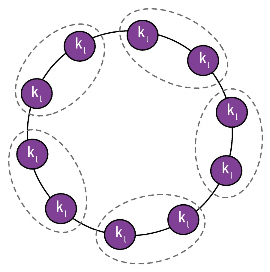
Image 9.18
Modularity Maxima
A ring network consisting of 24 cliques, each made of 5 nodes.
The Intuitive Partition
The best partition should correspond to the configuration where each cluster is a separate community. This partition has M=0.867
The Optimal Partition
If we combine the clusters into pairs, as illustrated by the node colors, we obtain M=0.871, higher than M obtained for the intuitive partition (a).
Random Partition
Partitions with comparable modularity tend to have rather distinct community structure. For example, if we assign each cluster randomly to communities, even clusters that have no links to each other, like the five highlighted clusters, may end up in the same community. The modularity of this random partition is still high, M=0.80, not too far from the optimal M=0.87.
Modularity Plateau
The modularity function of the network (a) reconstructed from 997 partitions. The vertical axis gives the modularity M, revealing a high-modularity plateau that consists of numerous low-modularity partitions. We lack, therefore, a clear modularity maxima - instead the modularity function is highly degenerate. After [40].
After [33].
In summary, modularity offers a first principle understanding of a network's community structure. Indeed, (9.16) incorporates in a compact form a number of essential questions, like what we mean by a community, how we choose the appropriate null model, and how we measure the goodness of a particular partition. Consequently modularity optimization plays a central role in the community finding literature.
At the same time, modularity has several well-known limitations: First, it forces together small weakly connected communities. Second, networks lack a clear modularity maxima, developing instead a modularity plateau containing many partitions with hard to distinguish modularity. This plateau explains why numerous modularity maximization algorithms can rapidly identify a high M partition: They identify one of the numerous partitions with close to optimal M. Finally, analytical calculations and numerical simulations indicate that even random networks contain high modularity partitions, at odds with the random hypothesis H3 that motivated the concept of modularity [41-43].
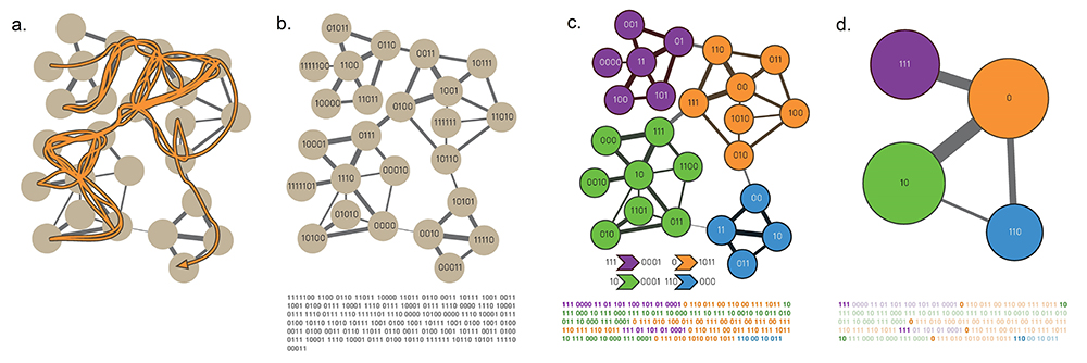
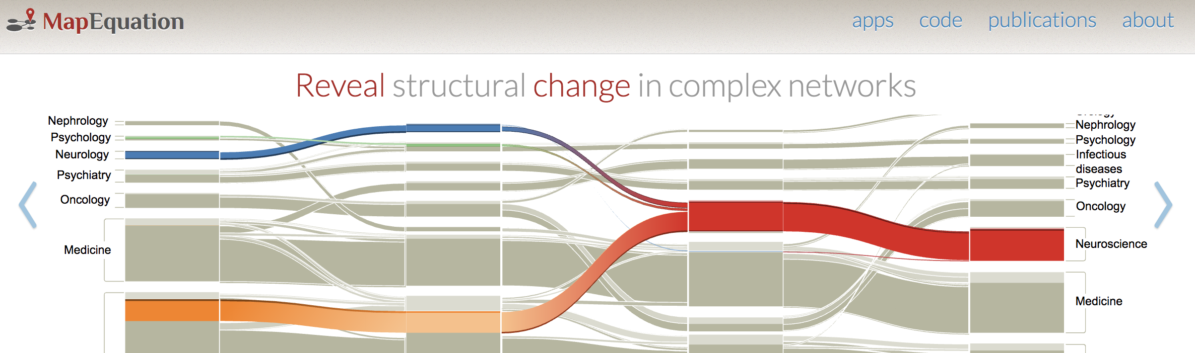
Modularity optimization is a special case of a larger problem: Finding communities by optimizing some quality function Q. The greedy algorithm and the Louvain algorithm described in ADVANCED TOPICS 9.C assume that Q = M, seeking partitions with maximal modularity. In ADVANCED TOPICS 9.C we also describe the Infomap algorithm, that finds communities by minimizing the map equation L, an entropy-based measure of the partition quality [44-46].
Section 9.5
Overlapping Communities
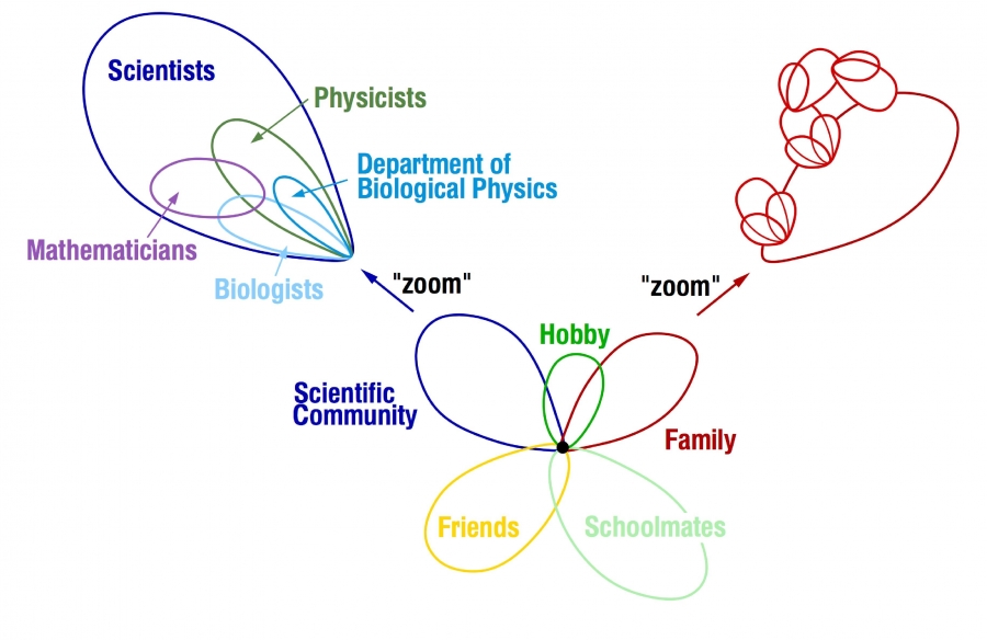
A node is rarely confined to a single community. Consider a scientist, who belongs to the community of scientists that share his professional interests. Yet, he also belongs to a community consisting of family members and relatives and perhaps another community of individuals sharing his hobby (Image 9.19). Each of these communities consists of individuals who are members of several other communities, resulting in a complicated web of nested and overlapping communities [36]. Overlapping communities are not limited to social systems: The same genes are often implicated in multiple diseases, an indication that disease modules of different disorders overlap [14].
Image 9.19
Overlapping Communities
Schematic representation of the communities surrounding Tamás Vicsek, who introduced the concept of overlapping communities. A zoom into the scientific community illustrates the nested and overlapping structure of the community characterizing his scientific interests. After [36].
While the existence of a nested community structure has long been appreciated by sociologists [47] and by the engineering community interested in graph partitioning, the algorithms discussed so far force each node into a single community. A turning point was the work of Tamás Vicsek and collaborators [36,48], who proposed an algorithm to identify overlapping communities, bringing the problem to the attention of the network science community. In this section we discuss two algorithms to detect overlapping communities, clique percolation and link clustering.
Online Resource 9.2 CFinder
The CFinder software, allowing us to identify overlapping communities, can be downloaded from www.cfinder.org.
Clique Percolation
The clique percolation algorithm, often called CFinder, views a community as the union of overlapping cliques [36]:
Two k-cliques are considered adjacent if they share k – 1 nodes (Image 9.20b).
A k-clique community is the largest connected subgraph obtained by the union of all adjacent k-cliques (Image 9.20c).
k-cliques that can not be reached from a particular k-clique belong to other k-clique communities (Image 9.20c,d).
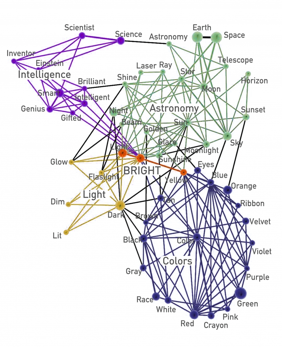
The CFinder algorithm identifies all cliques and then builds an Nclique x Nclique clique–clique overlap matrix O, where Nclique is the number of cliques and Oij is the number of nodes shared by cliques i and j (Image 9.39). A typical output of the CFinder algorithm is shown in Image 9.21, displaying the community structure of the word bright. In the network two words are linked to each other if they have a related meaning. We can easily check that the overlapping communities identified by the algorithm are meaningful: The word bright simultaneously belongs to a community containing light-related words, like glow or dark; to a community capturing colors (yellow, brown); to a community consisting of astronomical terms (sun, ray); and to a community linked to intelligence (gifted, brilliant). The example also illustrates the difficulty the earlier algorithms would have in identifying communities of this network: they would force bright into one of the four communities and remove from the other three. Hence communities would be stripped of a key member, leading to outcomes that are difficult to interpret.
Image 9.20
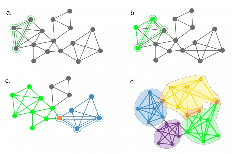
The Clique Percolation Algorithm (CFinder)
To identify k=3 clique-communities we roll a triangle across the network, such that each subsequent triangle shares one link (two nodes) with the previous triangle.
(a)-(b) Rolling Cliques
Starting from the triangle shown in green in (a), (b) illustrates the second step of the algorithm.
(c) Clique Communities for k=3
The algorithm pauses when the final triangle of the green community is added. As no more triangles share a link with the green triangles, the green community has been completed. Note that there can be multiple k-clique communities in the same network. We illustrate this by showing a second community in blue. The figure highlights the moment when we add the last triangle of the blue community. The blue and green communities overlap, sharing the orange node.
(d) Clique Communities for k=4 k=4 community structure of a small network, consisting of complete four node subgraphs that share at least three nodes. Orange nodes belong to multiple communities.
Images courtesy of Gergely Palla.
Could the communities identified by CFinder emerge by chance? To distinguish the real k-clique communities from communities that are a pure consequence of high link density we explore the percolation properties of k-cliques in a random network [48]. As we discussed in CHAPTER 3, if a random network is sufficiently dense, it has numerous cliques of varying order. A large k-clique community emerges in a random network only if the connection probability p exceeds the threshold (ADVANCED TOPICS 9.D)
Under pc(k) we expect only a few isolated k-cliques (Image 9.22a). Once p exceeds pc(k), we observe numerous cliques that form k-clique communities (Image 9.22b). In other words, each k-clique community has its own threshold:
For k=2 the k-cliques are links and (9.16) reduces to pc(k)~1/N, which is the condition for the emergence of a giant connected component in Erdős–Rényi networks.
For k =3 the cliques are triangles (Image 9.22a,b) and (9.16) predicts pc(k)~1/√2N.
Image 9.21
Overlapping Communities
Communities containing the word bright in the South Florida Free Association network, whose nodes are words, connected by a link if their meaning is related. The community structure identified by the CFinder algorithm accurately describes the multiple meanings of bright, a word that can be used to refer to light, color, astronomical terms, or intelligence. After [36].
In other words, k-clique communities naturally emerge in sufficiently dense networks. Consequently, to interpret the overlapping community structure of a network, we must compare it to the community structure obtained for the degree-randomized version of the original network.
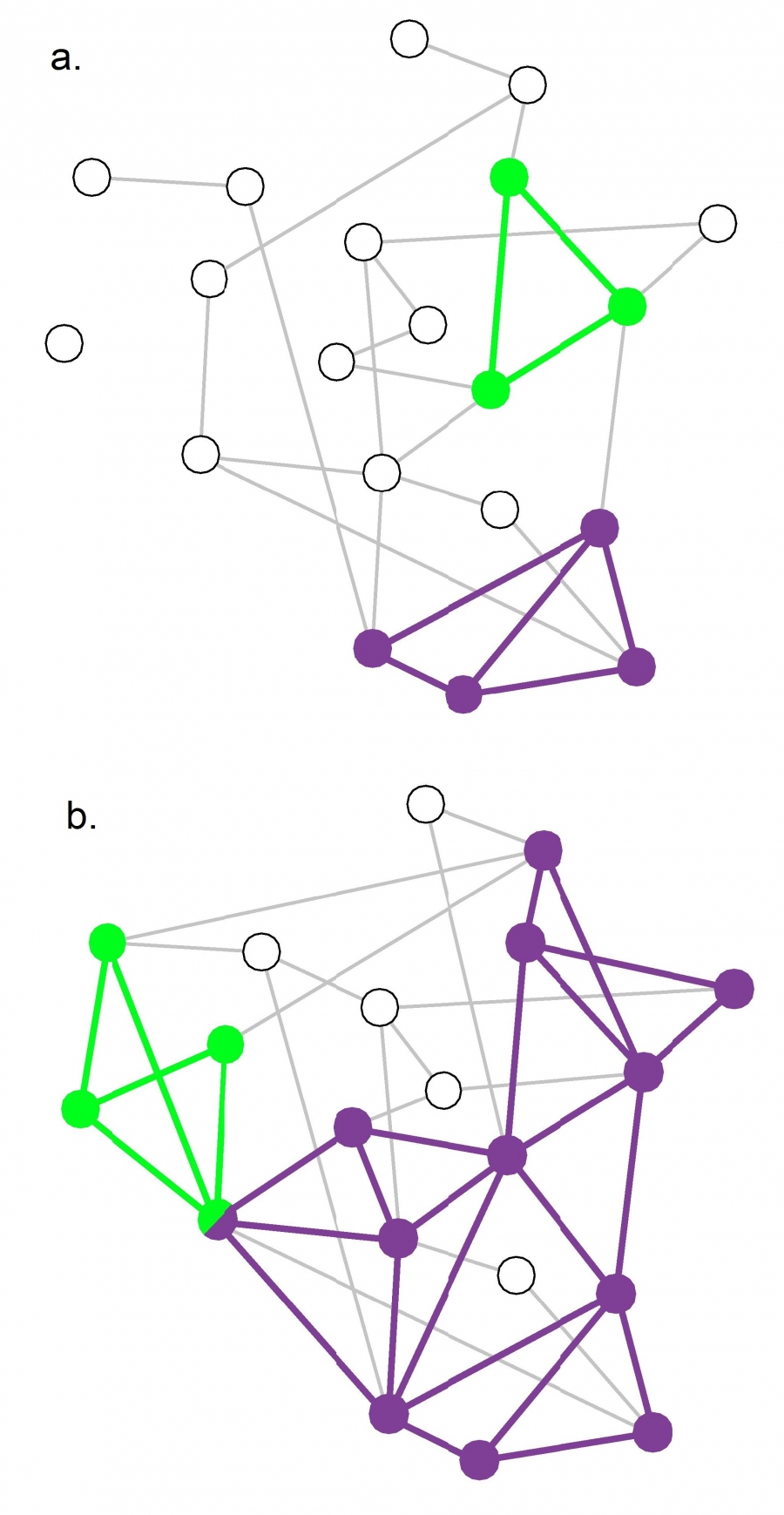
Image 9.22
The Clique Percolation Algorithm (CFinder)
Random networks built with probabilities p=0.13 (a) and p=0.22 (b). As both p's are larger than the link percolation threshold (pc=1/N=0.05 for N=20), in both cases most nodes belong to a giant component.
Subcritical Communities
The 3-clique (triangle) percolation threshold is pc(3)=0.16 according to (9.16), hence at p=0.13 we are below it. Therefore, only two small 3-clique percolation clusters are observed, which do not connect to each other.
Supercritical Communities
For p=0.22 we are above pc(3), hence we observe multiple 3-cliques that form a giant 3-clique percolation cluster (purple). This network also has a second overlapping 3-clique community, shown in green.
After [48].
Computational Complexity
Finding cliques in a network requires algorithms whose running time grows exponentially with N. Yet, the CFinder community definition is based on cliques instead of maximal cliques, which can be identified in polynomial time [49]. If, however, there are large cliques in the network, it is more efficient to identify all cliques using an algorithm with O(eN) complexity [36]. Despite this high computational complexity, the algorithm is relatively fast, processing the mobile call network of 4 million mobile phone users in less then one day [50] (see also Image 9.28).
Link Clustering
While nodes often belong to multiple communities, links tend to be community specific, capturing the precise relationship that defines a node’s membership in a community. For example, a link between two individuals may indicate that they are in the same family, or that they work together, or that they share a hobby, designations that only rarely overlap. Similarly, in biology each binding interaction of a protein is responsible for a different function, uniquely defining the role of the protein in the cell. This specificity of links has inspired the development of community finding algorithms that cluster links rather than nodes [51,52].
The link clustering algorithm proposed by Ahn, Bagrow and Lehmann [51] consists of the following steps:
Step 1: Define Link Similarity
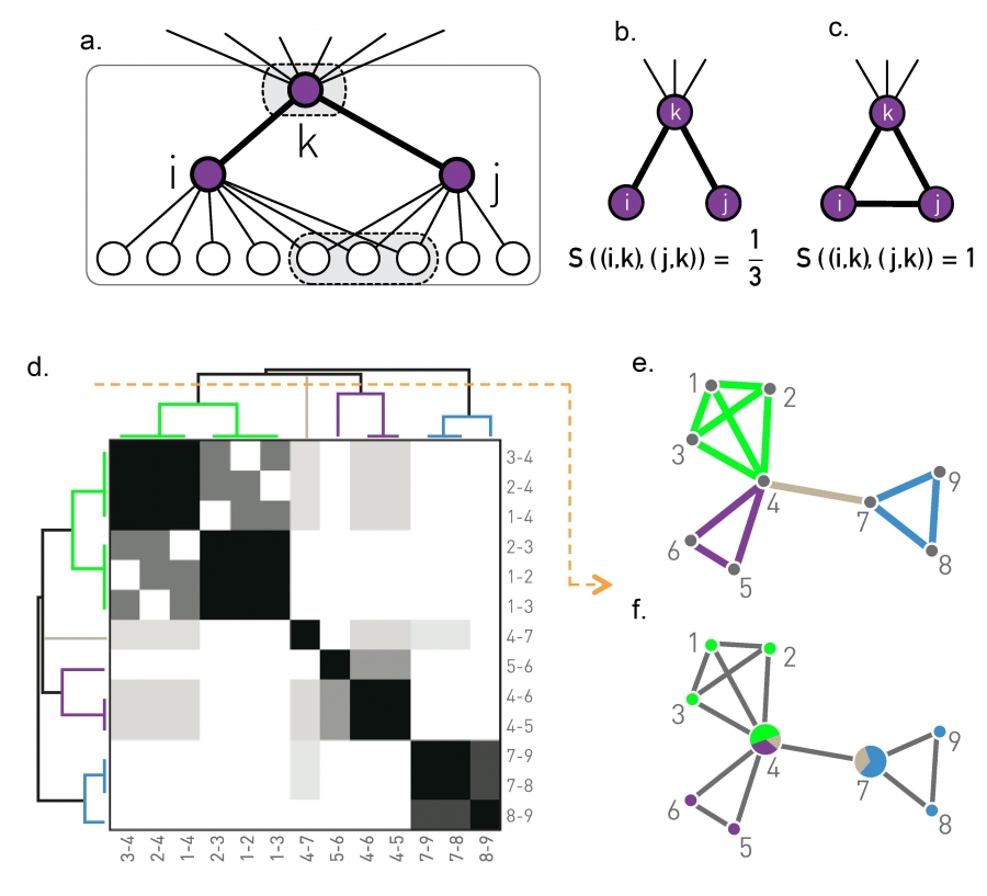
The similarity of a link pair is determined by the neighborhood of the nodes connected by them. Consider for example the links (i,k) and (j,k), connected to the same node k. Their similarity is defined as (Image 9.23a-c)
where n+(i) is the list of the neighbors of node i, including itself. Hence S measures the relative number of common neighbors i and j have. Consequently S=1 if i and j have the same neighbors (Image 9.23c). The less is the overlap between the neighborhood of the two links, the smaller is S (Image 9.23b).
Image 9.23
Identifying Link Communities
The link clustering algorithm identifies links with a similar topological role in a network. It does so by exploring the connectivity patterns of the nodes at the two ends of each link. Inspired by the similarity function of the Ravasz algorithm [4] (Image 9.19), the algorithm aims to assign to high similarity S the links that connect to the same group of nodes.
The similarity S of the (i,k) and (j,k) links connected to node k detects if the two links belong to the same group of nodes. Denoting with n+(i) the list of neighbors of node i, including itself, we obtain |n+(i)∪n+(j)| =12 and |n+(i)∩n+(j)| =4, resulting in S = 1/3 according to (9.17).
For an isolated (ki = kj = 1) connected triple we obtain S = 1/3.
For a triangle we have S = 1.
The link similarity matrix for the network shown in (e) and (f). Darker entries correspond to link pairs with higher similarity S. The figure also shows the resulting link dendrogram.
The link community structure predicted by the cut of the dendrogram shown as an orange dashed line in (d).
The overlapping node communities derived from the link communities shown in (e).
After [51].
Step 2: Apply Hierarchical Clustering
The similarity matrix S allows us to use hierarchical clustering to identify link communities (SECTION 9.3). We use a single-linkage procedure, iteratively merging communities with the largest similarity link pairs (Image 9.10).
Taken together, for the network of Image 9.23e, (9.17) provides the similarity matrix shown in (d). The single-linkage hierarchical clustering leads to the dendrogram shown in (d), whose cuts result in the link communities shown in (e) and the overlapping node communities shown in (f).
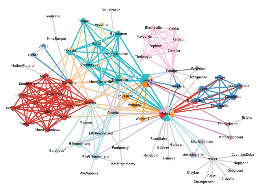
Image 9.24 illustrates the community structure of the characters of Victor Hugo’s novel Les Miserables identified using the link clustering algorithm. Anyone familiar with the novel can convince themselves that the communities accurately represent the role of each character. Several characters are placed in multiple communities, reflecting their overlapping roles in the novel. Links, however, are unique to each community.
Image 9.24
Link Communities
The network of characters in Victor Hugo’s 1862 novel Les Miserables. Two characters are connected if they interact directly with each other in the story. The link colors indicate the clusters, light grey nodes corresponding to single-link clusters. Nodes that belong to multiple communities are shown as pie-charts, illustrating their membership in each community. Not surprisingly, the main character, Jean Valjean, has the most diverse community membership. After [51].
Computational Complexity
The link clustering algorithm involves two time-limiting steps: similarity calculation and hierarchical clustering. Calculating the similarity (9.17) for a link pair with degrees ki and kj requires max(ki,kj) steps. For a scale-free network with degree exponent γ the calculation of similarity has complexity O(N2/(γ-1)), determined by the size of the largest node, kmax. Hierarchical clustering requires O(L2) time steps. Hence the algorithm's totalcomputational complexity is O(N2/(γ-1))+ O(L2). For sparse graphs the latter term dominates, leading to O(N2).
The need to detect overlapping communities have inspired numerous algorithms [53]. For example, the CFinder algorithm has been extended to the analysis of weighted [54], directed and bipartite graphs [55,56]. Similarly, one can derive quality functions for link clustering [52], like the modularity function discussed in SECTION 9.4.
In summary, the algorithms discussed in this section acknowledge the fact that nodes naturally belong to multiple communities. Therefore by forcing each node into a single community, as we did in the previous sections, we obtain a misleading characterization of the underlying community structure. Link communities recognize the fact that each link accurately captures the nature of the relationship between two nodes. As a bonus link clustering also predicts the overlapping community structure of a network.
Section 9.6
Testing Communities
Community identification algorithms offer a powerful diagnosis tool, allowing us to characterize the local structure of real networks. Yet, to interpret and use the predicted communities, we must understand the accuracy of our algorithms. Similarly, the need to diagnose large networks prompts us to address the computational efficiency of our algorithms. In this section we focus on the concepts needed to assess the accuracy and the speed of community finding.
Accuracy
If the community structure is uniquely encoded in the network’s wiring diagram, each algorithm should predict precisely the same communities. Yet, given the different hypotheses the various algorithms embody, the partitions uncovered by them can differ, prompting the question: Which community finding algorithm should we use?
To assess the performance of community finding algorithms we need to measure an algorithm’s accuracy, i.e. its ability to uncover communities in networks whose community structure is known. We start by discussing two benchmarks, which are networks with predefined community structure, that we can use to test the accuracy of a community finding algorithm.
Girvan-Newman (GN) Benchmark
The Girvan-Newman benchmark consists of N=128 nodes partitioned into nc=4 communities of size Nc=32 [9,57]. Each node is connected with probability pint to the Nc–1 nodes in its community and with probability pext to the 3Nc nodes in the other three communities. The control parameter
captures the density differences within and between communities. We expect community finding algorithms to perform well for small μ (Image 9.25a), when the probability of connecting to nodes within the same community exceeds the probability of connecting to nodes in different communities. The performance of all algorithms should drop for large μ (Image 9.25b), when the link density within the communities becomes comparable to the link density in the rest of the network.
Image 9.25
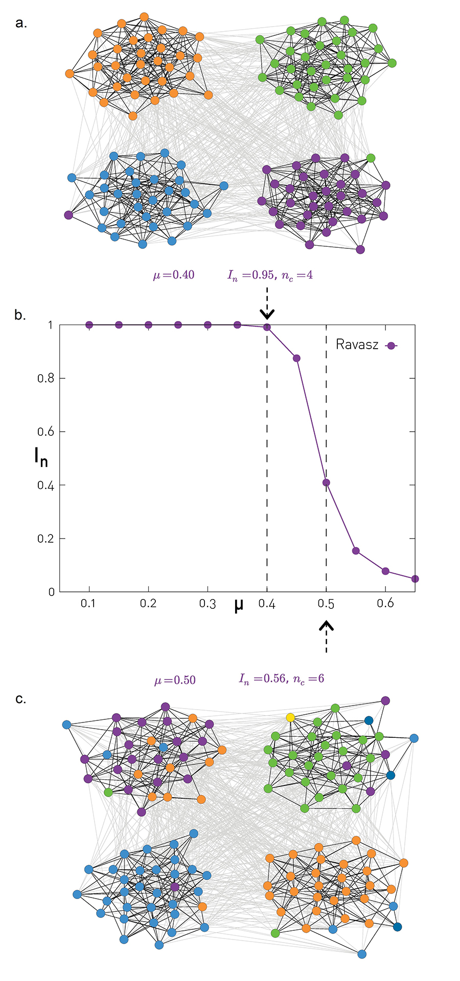
Testing Accuracy with the NG Benchmark
The position of each node in (a) and (c) shows the planted communities of the Girvan-Newman (GN) benchmark, illustrating the presence of four distinct communities, each with Nc=32 nodes.
The node colors represent the partitions predicted by the Ravasz algorithm for mixing parameter μ=0.40 given by (9.18). As in this case the communities are well separated, we have an excellent agreement between the planted and the detected communities.
The normalized mutual information in function of the mixing parameter μ for the Ravasz algorithm. For small μ we have In≃1 and nc, indicating that the algorithm can easily detect well separated communities, as illustrated in (a). As we increase μ the link density difference within and between communities becomes less pronounced. Consequently the communities are increasingly difficult to identify and In decreases.
For μ=0.50 the Ravasz algorithm misplaces a notable fraction of the nodes, as in this case the communities are not well separated, making it harder to identify the correct community structure
Note that the Ravasz algorithm generates multiple partitions, hence for each μ we show the partition with the largest modularity, M. Next to (a) and (c) we show the normalized mutual information associated with the corresponding partition and the number of detected communities nc. The normalized mutual information (9.23), developed for non-overlapping communities, can be extended to overlapping communities as well [59].
Lancichinetti-Fortunato-Radicchi (LFR) Benchmark
The GN benchmark generates a random graph in which all nodes have comparable degree and all communities have identical size. Yet, the degree distribution of most real networks is fat tailed, and so is the community size distribution (Image 9.29). Hence an algorithm that performs well on the GN benchmark may not do well on real networks. To avoid this limitation, the LFR benchmark (Image 9.26) builds networks for which both the node degrees and the planted community sizes follow power laws [58].
Having built networks with known community structure, next we need tools to measure the accuracy of the partition predicted by a particular community finding algorithm. As we do so, we must keep in mind that the two benchmarks discussed above correspond to a particular definition of communities. Consequently algorithms based on clique percolation or link clustering, that embody a different notion of communities, may not fare so well on these.
Image 9.26
LFR Benchmark
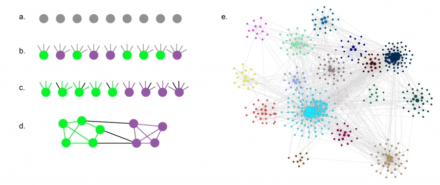
The construction of the Lancichinetti-Fortunato-Radicchi (LFR) benchmark, which generates networks in which both the node degrees and community sizes follow a power law. The benchmark is built as follows [57]:
Start with N isolated nodes.
Assign each node to a community of size Nc where Nc follows the power law distribution PNc~Nc-ζ with community exponent ζ. Also assign each node i a degree ki selected from the power law distribution pk~k-γ with degree exponent γ.
Each node i of a community receives an internal degree (1-μ)ki, shown as links whose color agrees with the node color. The remaining μki degrees, shown as black links, connect to nodes in other communities.
All stubs of nodes of the same community are randomly attached to each other, until no more stubs are ‘‘free’’. In this way we maintain the sequence of internal degrees of each node in its community. The remaining μki stubs are randomly attached to nodes from other communities
A typical network and its community structure generated by the LFR benchmark with N=500, γ=2.5, and ζ=2.
Measuring Accuracy
To compare the predicted communities with those planted in the benchmark, consider an arbitrary partition into non-overlapping communities. In each step we randomly choose a node and record the label of the community it belongs to. The result is a random string of community labels that follow a p(C) distribution, representing the probability that a randomly selected node belongs to the community C.
Consider two partitions of the same network, one being the benchmark (ground truth) and the other the partition predicted by a community finding algorithm. Each partition has its own p(C1) and p(C2) distribution. The joint distribution, p(C1, C2), is the probability that a randomly chosen node belongs to community C1 in the first partition and C2 in the second. The similarity of the two partitions is captured by the normalized mutual information [38]
The numerator of (9.19) is the mutual information I, measuring the information shared by the two community assignments: I=0 if C1 and C2 are independent of each other; I equals the maximal value H({p(C1)}) = H({p(C2)}) when the two partitions are identical and is the Shannon entropy.
If all nodes belong to the same community, then we are certain about the next label and H=0, as we do not gain new information by inspecting the community to which the next node belongs to. H is maximal if p(C) is the uniform distribution, as in this case we have no idea which community comes next and each new node provides H bits of new information.
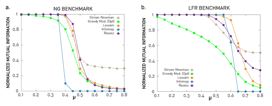
In summary, In=1 if the benchmark and the detected partitions are identical, and In=0 if they are independent of each other. The utility of In is illustrated in Image 9.25b that shows the accuracy of the Ravasz algorithm for the Girvan-Newman benchmark. In Image 9.27 we use In to test the performance of each algorithm against the GN and LFR benchmarks. The results allow us to draw several conclusions:
We have In≃1 for μ < 0.5. Consequently when the link density within communities is high compared to their surroundings, most algorithms accurately identify the planted communities. Beyond μ=0.5 the accuracy of each algorithm drops.
The accuracy is benchmarks dependent. For the more realistic LFR benchmark the Louvain and the Ravasz methods offer the best performance and greedy modularity performs poorly.
Image 9.27
Testing Against Benchmarks
We tested each community finding algorithm that predicts non-overlapping communities against the GN and the LFR benchmarks. The plots show the normalized mutual information In against μ for five algorithms. For the naming of each algorithm, see Table 9.1.
Start with N isolated nodes.
GN Benchmark
The horizontal axis shows the mixing parameter (9.18), representing the fraction of links connecting different communities. The vertical axis is the normalized mutual information (9.19). Each curve is averaged over 100 independent realizations.
LFR Benchmark
Same as in (a) but for the LFR benchmark. The benchmark parameters are N=1,000, 〈k〉=20, γ=2, kmax=50, ζ=1, maximum community size: 100, minimum community size: 20. Each curve is averaged over 25 independent realizations.
Speed
As discussed in SECTION 9.2, the number of possible partitions increases faster than exponentially with N, becoming astronomically high for most real networks. While community identification algorithms do not check all partitions, their computational cost still varies widely, determining their speed and consequently the size of the network they can handle. Table 9.1 summarizes the computational complexity of the algorithms discussed in this chapter. Accordingly, the most efficient are the Louvain and the Infomap algorithms, both of which scale as 0(NlogN). The least efficient is CFinder with 0(eN).
Table 9.1
Algorithmic Complexity
The computational complexity of the community identification algorithms discussed in this chapter. While computational complexity depends on both N and L, for sparse networks with good approximation we have L~N. We therefore list computational complexity in terms of N only.
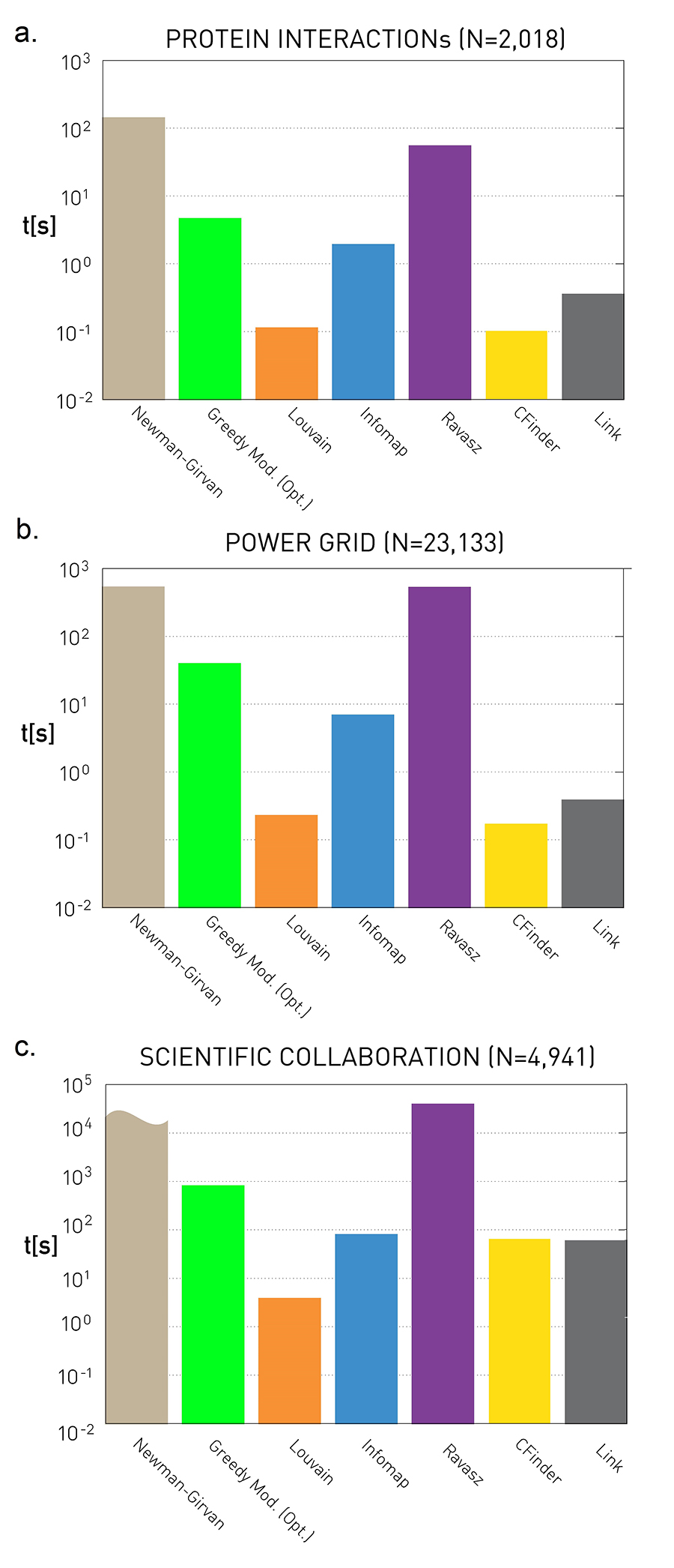
These scaling laws do not capture the actual running time, however. They only show how the running time scales with N. This scaling matters if we need to find communities in very large networks. To get a sense of the true speed of these algorithms we measured their running time for the protein interaction network (N=2,018), the power grid (N=4,941) and the scientific collaboration network (N=23,133), using the same computer. The results, shown in Image 9.28, indicate that:
The Louvain method requires the shortest running time for all networks. CFinder is just as fast for the mid-size networks, and its running time is comparable to the other algorithms for the larger collaboration network.
The Girvan-Newman algorithm is the slowest on each network, in line with its predicted high computational complexity (Table 9.1). For example the algorithm failed to find communities in the scientific collaboration network in seven days.
In summary, benchmarks allow us to compare the accuracy and the speed of the available algorithms. Given that the development of the fastest and the most accurate community detection tool remains an active arms race, those interested in the subject should consult the literature that compares algorithms across multiple dimensions [31,58,60,61].
Image 9.28
The Running Time
To compare the speed of community detection algorithms we used their python implementation, either relying on the versions published by their developers or the available implementation in the igraph software package. The Ravasz algorithm was implemented by us, hence it is not optimized, having a larger running time than ideally possible. We ran each algorithm on the same computer. The plots provide their running time in seconds for three real networks. For the science collaboration network the Newman-Girvan algorithm did not finish after seven days, hence we only provide the lower limit of its running time. The higher running time observed for the scientific collaboration network is rooted in the larger size of this network.
Section 9.7
Characterizing Communities
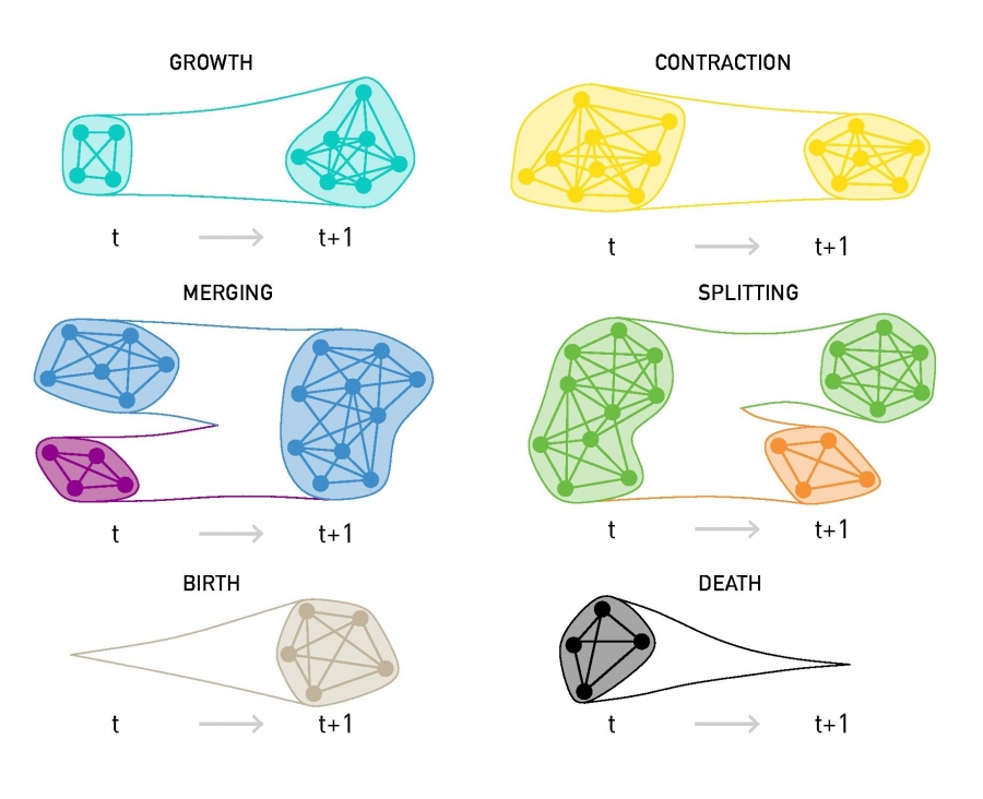
Research in network science is driven by the desire to quantify the fundamental principles that govern how networks emerge and how they are organized. These organizing principles impact the structure of communities, as well as our ability to identify them. In this section we discuss community evolution, the characteristics of community size distribution and the role of the link weights in community identification, allowing us to uncover the generic principles of community organization.
Community Size Distribution
According to the fundamental hypothesis (H1) the number and the size of communities in a network are uniquely determined by the network’s wiring diagram. We must therefore ask: What is the size distribution of these communities?
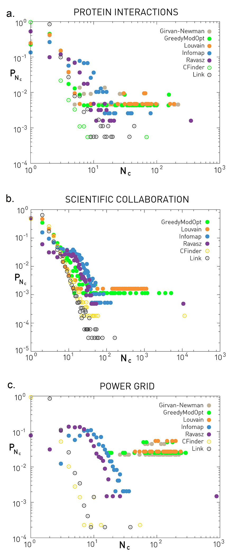
Many studies report fat tailed community size distributions, implying that numerous small communities coexist with a few very large ones [16,33,35,36,60]. To explore how widespread this pattern is, in Figure 9.29 we show pNc for three networks, as predicted by various community finding algorithms. The plots indicate several patterns:
For the protein interaction and the science collaboration network all algorithms predict an approximately fat tailed pNc. Hence in these networks numerous tiny communities coexist with a few large communities.
For the power grid different algorithms lead to distinct outcomes. Modularity-based algorithms predict communities with comparable size Nc ≃ 102. In contrast, the Ravasz algorithm and Infomap predict numerous communities with size Nc ≃ 10 and a few larger communities. Finally, clique percolation and link clustering predict an approximately fat tailed community size distribution.
These differences suggest that the fat tailed community size distribution is not a byproduct of a particular algorithm. Rather it is an inherent property of some networks, like the protein and the scientific collaboration network. The different outcomes for the power grid suggests that this network lacks a unique and detectable community structure.
Image 9.29
Community Size Distribution
The community size distribution pNc predicted by the community finding algorithms explored in this chapter. The name convention for the algorithms is shown in Table 9.1. For the protein interaction (a) and the scientific collaboration network (b) all algorithms predict an approximately fat-tailed community size distribution, hence the predictions are more-or-less consistent with each other. The algorithms offer conflicting results for the power grid, shown in (c).
Communities and Link Weights
Link weights are deeply correlated with the community structure. Yet, as we discuss next, the nature of these correlations is system dependent.
Social Networks
The more time two individuals spend together, the more likely that they share friends, which increases the chance that they belong to the same community. Consequently communities in social networks tend to be nucleated around strong ties. Links connecting different communities are weaker in comparison. This pattern, known as the weak tie hypothesis [62], is illustrated in Image 9.30a for the mobile call network [63]. We observe that strong ties are indeed predominantly within the numerous small communities, and links connecting communities are visibly weaker.
Transport Systems
The purpose of many technological and biological networks is to transport materials or information. In this case the link weights are expected to correlate with betweenness centrality [64,65,66], a proxy of the local traffic carried by a network. As links connecting different communities must transport considerable amount of traffic, in transport networks strong ties are between communities. In contrast links within communities are weaker in comparison (Image 9.30b).
The coupling between link weights and community structure suggests that incorporating the link weights could enhance the accuracy of community finding algorithms. Yet, the different nature of the coupling in social and technological systems serves as a cautionary note: Algorithms that aim to place in the same community nodes connected by strong ties may be only effective in social systems. They may offer potentially misleading results in technological and biological systems, where strong ties connect different communities.
Image 9.30
Communities and Link Weights
The mobile call network helps us illustrate the relationship between link weights and communities. Links represent mutual calls between the users. We show only nodes that are at distance six or less from the individual highlighted as a black circle in (a).
Real Weights
The link colors capture the aggregate call duration in minutes (see color bar). In line with the weak tie hypothesis we find strong ties mainly within communities and weak ties between communities [62].
Betweenness Centrality
If the link weights are driven by the need to transport information or materials, as it is often the case in technological and biological systems, the weights are well approximated by betweenness centrality (Image 9.11). We colored the links based on each link’s betweenness centrality. As the figure indicates, links connecting communities have high betweenness (red), whereas the links within communities have low betweenness (green).
Community Evolution
Changes in a network’s wiring diagram can have multiple consequences for communities: they can lead to the birth of new communities, the growth or the contraction of the existing communities, communities can merge with each other or split into several smaller communities, and finally communities can die (Image 9.31) [50]. Studies focusing on social and communication networks offer several insights into the changes communities experience [50,67-73]:
Growth
The probability that a node joins a community grows with the number of links the node has to members of that community [73].
Contraction
Nodes with only a few links to members of their community are more likely to leave the community than nodes with multiple links to community members [73]. In weighted networks the probability that a node leaves a community increases with the sum of its link weights to nodes outside the community.
Splitting or Death
The probability that a community disintegrates increases with the aggregate link weights to nodes outside the community.
Age
There is positive correlation between the age of a community and its size, indicating that older communities tend to be larger [50].
Community Stability
The membership of large communities changes faster with time than the membership of smaller communities. Indeed, in social networks large communities often correspond to institutions, companies or schools, that renew themselves by accepting new members, hiring new employees or enrolling new students. For small communities stability requires stable membership [50].
These results were obtained in the context of social systems. Our understanding of the patterns that cover community evolution in technological or biological systems remains limited.
Image 9.31
Evolving Communities
When networks evolve in time, so does the underlying community structure. All changes in community structure are the result of six elementary events in the life of a community, illustrated in the figure: a community can grow or contract; communities can merge or may split; new communities are born while others may disappear. After [50].
In summary, several recurring patterns characterize the organization and the evolution of communities. The community size distribution is typically fat tailed, indicating the coexistence of many small communities with a few large ones. We also find system-dependent correlations between the community structure and link weights, so that in social systems the strong ties are mainly within communities, while in transport systems they are between communities. Finally, we gained an increasing understanding of the dynamical patterns that govern community evolution.
Section 9.8
Summary
The ubiquity of communities across different networks has turned community identification into a dynamically developing chapter of network science. Many of the developed algorithms are now available as software packages, allowing their immediate use for network diagnosis. Yet, the efficient use of these algorithms and the interpretation of their predictions requires us to be aware of the assumptions built into them. In this chapter we provided the intellectual and the quantitative foundations of community detection, helping us understand the origin and the assumptions behind the most frequently used algorithms.
Despite the successes of community identification, the field is faced with numerous open questions:
Do We Really Have Communities?
Throughout this chapter we avoided a fundamental question: How do we know that there are indeed communities in a particular network? In other words, could we decide that a network has communities without first identifying the communities themselves? The lack of an answer to this question represents perhaps the most glaring gap of the community finding literature. Community finding algorithms are designed to identify communities, whether they are there or not.
Hypotheses or Theorems?
Community identification relies on four hypotheses, summarized in BOX 9.3. We call them hypotheses because we can not prove their correctness. Further advances might be able to turn the Fundamental, the Random and the Maximal Modularity Hypotheses into theorems. Or we may learn about their limitations, as we did in the case of the Maximal Modularity Hypothesis (SECTION 9.6).
Must all Nodes Belong to Communities?
Community detection algorithm force all nodes into communities. This is likely an overkill for most real networks: some nodes belong to a single community, others to multiple communities, and likely many nodes do not belong to any community. Most algorithms used in community identification do not make this distinction, forcing instead all nodes into some community.
Dense vs. Sparse Communities
Most networks explored in this book are sparse. Yet, with improvements in data collection, many real network maps will likely gain numerous links. In dense networks we often see numerous highly overlapping communities, forcing us to reevaluate the validity of the various hypotheses, and the appropriateness of the community detection algorithms discussed in this chapter. For example, in highly overlapping communities nodes may have higher external than internal degrees, limiting the validity of the density hypothesis.
Do Communities Matter?
We resort to an example to answer this question. Image 9.32a shows a local neighborhood of the mobile call network, highlighting four communities identified by the link clustering algorithm (SECTION 9.5). The figure also shows the call frequency at noon (b) and at midnight (c), documenting different calling habits at different parts of the day. We find that the members of the top right community, shown as brown nodes in (a), are active at midnight (b), but they stop calling each other at noon (c). In contrast the light and the dark blue communities are active at noon, but are sleepy at midnight. This indicates that communities, identified only from the network’s wiring diagram, have coherent community-specific activity patterns.
Image 9.32
Communities and Call Patterns
The direct impact of communities on the activity of their members is illustrated by the mobile call network, offering us simultaneous information on community structure and user activity.
Community Structure
Four communities of the mobile phone network, each community being colored differently. These communities represent local neighborhoods in the call patterns of over one million consumers, as predicted by the link clustering algorithm (SECTION 9.5). The rest of the mobile phone network is not shown.
Midnight Activity
The calling patterns of the users in the four communities shown in (a). The link colors reflect the frequency of calls in the hourlong interval around midnight. Red links signal numerous calls around midnight; white or missing links imply that the users talked little or did not call each other in this time frame.
Noon Activity
The same as in (b) but at noon.
Image courtesy of Sune Lehmann.
Image 9.32 suggests that once present, communities have a profound impact on network behavior. Numerous measurements support this conclusion: Information travels fast within a community but has difficulty reaching other communities [63]; communities influence the link weights [62]; the presence of communities can lead to degree correlations [74].
Communities are equally remarkable for their potential applications. For example, strengthening the links between clients that belong to the same community on the WWW can improve the performance of Webbased services [75]. In marketing, community finding can be used to identify customers with similar interests or purchasing habits, helping design efficient product recommendation systems [76]. Communities are often used to create data structures that can handle queries in a timely fashion [77,78]. Finally, community finding algorithms run behind many social networks sites, like Facebook, Twitter, or LinkedIn, helping these services discover potential friends, posts of interests and target advertising.
While community finding has deep roots in social and computer science, it is a relatively young chapter of network science (BOX 9.4). As such, our understanding of community organization continues to develop rapidly, offering increasingly accurate tools to diagnose the local structure of large networks.
Section 9.9
Homework
Hierarchical Networks
Calculate the degree exponent of the hierarchical network shown in Image 9.33.
Image 9.33
Hierarchical Networks
The colors represent the subsequent stages of the network's construction.
Communities on a Circle
Consider a one dimensional lattice with N nodes that form a circle, where each node connects to its two neighbors. Partition the line into nc consecutive clusters of size Nc=N/nc.
Calculate the modularity of the obtained partition.
According to the Maximum Modularity Hypothesis (SECTION 9.4), the maximum of Mc corresponds to the best partition. Obtain the community size nc corresponding to the best partition.
Modularity Resolution Limit
Consider a network consisting of a ring of nc cliques, each clique having Nc nodes and m(m–1)/2 links. The neighboring cliques are connected by a single link (Image 9.34). The network has an obvious community structure, each community corresponding to a clique.
Determine the modularity Msingle of this natural partition, and the modularity Mpairs of the partition in which pairs of neighboring cliques are merged into a single community, as indicated by the dotted lines in Image 9.34.
Show that only for nc < 2L will the modularity maximum predict the intuitively correct community partition, where
Discuss the consequences of violating the above inequality.
Modularity Maximum.
Show that the maximum value of modularity M defined in (9.12) cannot exceed one.
In this section we discuss the scaling properties of the hierarchical model introduced in Image 9.13. We calculate the degree distribution and the degree-dependent clustering coefficient, deriving (9.8). Finally, we explore the presence of hierarchy in the ten real networks.
Image 9.35
Calculating the degree exponent
The structure of a hierarchical network and the naming convention we use to refer to the hubs. After [11].
Degree Distribution
To compute the model's degree distribution we count the nodes with different degrees. Starting with the five nodes of the first module in Image 9.13a, we label the middle one a hub and call the remaining four nodes peripheral. All copies of this hub are again called hubs and we continue calling copies of peripheral nodes peripheral (Image 9.35).
The largest hub at the center of the network acquires 4n links during the nth iteration. Let us call this central hub Hn and the four copies of this hub Hn–1 (Image 9.35). We call Hn–2 the 4 · 5 leftover module centers whose size equals the size of the network at the (n–2)th iteration.
At the nth iteration the degree of the hub Hi follows
where we used
or
For i < n the number of Hi modules is
i.e. there are four modules for i = n – 1; 4 · 5 modules for i = n – 2; ...; and 4 · 5 n–2 for i=n. Since we have 4 · 5 n–i–1Hi-type hubs of degree kn(Hi), (4.35) and (4.38) allow us to write
where
Note that in (9.40) we used the approximation 4i–1≃4i.
For all k > n + 2 we can combine (9.40) and (9.41) to obtain
or
To calculate the degree distribution we need to normalize Nn(Hi) by calculating the ratio
Using
we obtain
In other words the obtained hierarchical network’s degree exponent is
Clustering Coefficient
It is somewhat straightforward to calculate the clustering coefficient of the Hi hubs. Their Σil=14l links come from nodes linked in a square, thus the connections between them equals their number. Consequently the number of links between the Hi’s neighbors is
providing
In other words we obtain
indicating that C(k) for the hubs scales as k–1, in line with (9.8).
Empirical Results Image 9.36 shows the C(k) function for the ten reference networks. We also show C(k) for each network after we applied degree-preserving randomization (green symbols), allowing us to make several observations:
For small k all networks have an order of magnitude higher C(k) than their randomized counterpart. Therefore the small degree nodes are located in much denser neighborhoods than expected by chance.
For the scientific collaboration, metabolic, and citation networks with a good approximation we have C(k)~k–1, while the randomized C(k) is flat. Hence these networks display the hierarchical modularity of the model of Image 9.13.
For the Internet, mobile phone calls, actors, email, protein interactions and the WWW C(k) decreases with k, while their randomized C(k) is k-independent. Hence while these networks display a hierarchical modularity, the observed C(k) is not captured by our simple hierarchical model. To fit the C(k) of these systems we need to build models that accurately capture their evolution. Such models predict that C(k)~k–β, where β can be different from one [27].
Only for the power grid we observe a flat, k-independent C(k), indicating the lack of a hierarchical modularity.
Taken together, Image 9.36 indicates that most real networks display some nontrivial hierarchical modularity.
Image 9.36
Hierarchy in Real Networks
The scaling of C(k) with k for the ten reference networks (purple symbols). The green symbols show C(k) obtained after applying degree preserving randomization to each network, that washes out the local density fluctuations. Consequently communities and the underlying hierarchy are gone. Directed networks were made undirected to measure C(k). The dashed line in each figure has slope -1, following (9.8), serving as a guide to the eye.
In this section we derive the expressions (9.12) and (9.13), characterizing the modularity fuction and its changes.
Modularity as a Sum Over Communities
Using (9.9) and (9.10) we can write the modularity of a full network as
where Ci is the label of the community to which node i belongs to. As only node pairs that belong to the same community contribute to the sum in (9.51), we can rewrite the first term as a sum over communities,
where Lc is the number of links within community Cc. The factor 2 disappears because each link is counted twice in Aij.
In a similar fashion the second term of (9.51) becomes
where kc is the total degree of the nodes in community Cc. Indeed, in the configuration model the probability that a stub connects to a randomly chosen stub is 1/2L, as in total we have 2L stubs in the network. Hence the likelihood that our stub connects to a stub inside the module is kc/2L. By repeating this procedure for all kc stubs within the community Cc and adding 1/2 to avoid double counting, we obtain the last term of (9.53).
Combining (9.52) and (9.53) leads to (9.12).
Merging Two Communities
Consider communities A and B and denote with kA and kB the total degree in these communities (equivalent with kc above). We wish to calculate the change in modularity after we merge these two communities. Using (9.12), this change can be written as
where
lAB is the number of direct links between the nodes of communities A and B, and
After inserting (9.55) and (9.56) into (9.54), we obtain
which is (9.13).
Section 9.12
Advanced Topic 9.C Fast Algorithms for Community Detection
The algorithms discussed in this chapter were chosen to illustrate the fundamental ideas and concepts pertaining to community detection. Consequently they are not guaranteed to be neither the fastest nor the most accurate algorithms. Recently two algorithms, called the Louvain algorithm and Infomap have gained popularity, as their accuracy is comparable to the accuracy of the algorithms covered in this chapter but offer better scalability. Consequently we can use them to identify communities in very large networks.
There are many similarities between the two algorithms:
They both aim to optimize a quality function Q . For the Louvain algorithm Q is modularity, M, and for Infomap Q is an entropy-based measure called the map equation or L.
Both algorithms use the same optimization procedure.
Given these similarities, we discuss the algorithms together.
The Louvain Algorithm
The O(N2) computational complexity of the greedy algorithm can be prohibitive for very large networks. A modularity optimization algorithm with better scalability was proposed by Blondel and collaborators [2]. The Louvain algorithm consists of two steps that are repeated iteratively (Image 9.37):
Step I
Start with a weighted network of N nodes, initially assigning each node to a different community. For each node i we evaluate the gain in modularity if we place node i in the community of one of its neighbors j. We then move node i in the community for which the modularity gain is the largest, but only if this gain is positive. If no positive gain is found, i stays in its original community. This process is applied to all nodes until no further improvement can be achieved, completing Step I.
The modularity change ΔM obtained by moving an isolated node i into a community C can be calculated using
where Σin is the sum of the weights of the links inside C (which is LC for an unweighted network); Σtot is the sum of the link weights of all nodes in C; ki is the sum of the weights of the links incident to node i; ki,in is the sum of the weights of the links from i to nodes in C and W is the sum of the weights of all links in the network.
Note that ΔM is a special case of (9.13), which provides the change in modularity after merging communities A and B. In the current case B is an isolated node. We can use ΔM to determine the modularity change when i is removed from the community it belonged earlier. For this we calculate ΔM for merging i with the community C after we excluded i from it. The change after removing i is –ΔM.
Step II
We construct a new network whose nodes are the communities identified during Step I. The weight of the link between two nodes is the sum of the weight of the links between the nodes in the corresponding communities. Links between nodes of the same community lead to weighted self-loops.
Once Step II is completed, we repeat Steps I - II, calling their combination a pass (Image 9.37). The number of communities decreases with each pass. The passes are repeated until there are no more changes and maximum modularity is attained.
Image 9.37
The Louvain Algorithm
The main steps of the Louvain algorithm. Each pass consists of two distinct steps:
Step I
Modularity is optimized by local changes. We choose a node and calculate the change in modularity, (9.58), if the node joins the community of its immediate neighbors. The figure shows the expected modularity change ΔMo,i for node 0. Accordingly node 0 will join node 3, as the modularity change for this move is the largest, being ΔM0,3=0.032. This process is repeated for each node, the node colors corresponding to the resulting communities, concluding Step I.
Step II
The communities obtained in Step I are aggregated, building a new network of communities. Nodes belonging to the same community are merged into a single node, as shown on the top right. This process will generate self-loops, corresponding to links between nodes in the same community that are now merged into a single node.
The sum of Steps I & II are called a pass. The network obtained after each pass is processed again (Pass 2), until no further increase of modularity is possible. After [2].
Computational Complexity
The Louvain algorithm is more limited by storage demands than by computational time. The number of computations scale linearly with L for the most time consuming first pass. With subsequent passes over a decreasing number of nodes and links, the complexity of the algorithm is at most O(L). It therefore allows us to identify communities in networks with millions of nodes.
Infomap
Introduced by Martin Rosvall and Carl T Bergstrom, Infomap exploits data compression for community identification (Image 9.38) [44-46]. It does it by optimizing a quality function for community detection in directed and weighted networks, called the map equation.
Consider a network partitioned into nc communities. We wish to encode in the most efficient fashion the trajectory of a random walker on this network. In other words, we want to describe the trojectory with the smallest number of symbols. The ideal code should take advantage of the fact that the random walker tends to get trapped into communities, staying there for a long time (Image 9.38c).
To achieve this coding we assign:
One code to each community (index codebook). For example the purple community in Image 9.38c is assigned the code 111.
Codewords for each node within each community. For example the top left node in (c) is assigned 001. Note that the same node code can be reused in different communities.
Exit codes that mark when the walker leaves a community, like 0001 for the purple community in (c).
Image 9.38
From Data Compression to Communities
Infomap detect communities by compressing the movement of a random walker on a network.
The orange line shows the trajectory of a random walker on a small network. We want to describe this trajectory with a minimal number of symbols, which we can achieve by assigning repeatedly used structures (communities) short and unique names.
We start by giving a unique name to each node. This is derived using a Huffman coding, a data compression algorithm that assigns each node a code using the estimated probability that the random walk visits that node. The 314 bits under the network describe the sample trajectory of the random walker shown in (a), starting with 1111100 for the first node of the walk in the upper left corner, 1100 for the second node, etc., and ending with 00011 for the last node on the walk in the lower right corner.
The figure shows a two-level encoding of the random walk, in which each community receives a unique name, but the name of nodes within communities are reused. This code yields on average a 32% shorter coding. The codes naming the communities and the codes used to indicate an exit from each community are shown to the left and the right of the arrows under the network, respectively. Using this code, we can describe the walk in (a) by the 243 bits shown under the network in (c). The first three bits 111 indicate that the walk begins in the red community, the code 0000 specifies the first node of the walk, etc.
By reporting only the community names, and not the locations of each node within the communities, we obtain an efficient coarse graining of the network, which corresponds to its community structure.
The goal, therefore, is to build a code that offers the shortest description of the random walk. Once we have this code, we can identify the network's community structure by reading the index codebook, which is uniquely assigned to each community (Image 9.38c).
The optimal code is obtained by finding the minimum of the map equation
In a nutshell, the first term of (9.59) gives the average number of bits necessary to describe the movement between communities where q is the probability that the random walker switches communities during a given step.
The second term gives the average number of bits necessary to describe movement within communities. Here H(Pc) is the entropy of within-community movements — including an “exit code” to capture the departure from a community i.
The specific terms of the maps equation and their calculation in terms of the probabilities capturing the movement of a random walker on a network, is somewhat involved. They are described in detail in Ref [44-46]. Online Resource 9.3 offers an interactive tool to illustrate the mechanism behind (9.59) and its use.
Online Resource 9.3 Map Equation for Infomap
For a dynamic visualization of the mechanism behind the map equation, see http://www.tp.umu. se/~rosvall/livemod/mapequation/.
At the end L serves as a quality function, that takes up a specific value for a particular partition of the network into communities. To find the best partition, we must minimize L over all possible partitions. The popular implementation of this optimization procedure follows Steps I and II of the Louvain algorithm: We assign each node to a separate community, and we systematically join neighboring nodes into modules if the move decreases L. After each move L is updated using (9.59). The obtained communities are joined into supercommunities, finishing a pass, after which the algorithm is restarted on the new, reduced network.
Computational Complexity
The computational complexity of Infomap is determined by the procedure used to minimize the map equation L. If we use the Louvain procedure, the computational complexity is the same as that of the Louvain algorithm, i.e. at most O(LlogL) or O(NlogN) for a sparse graph.
In summary, the Louvain algorithm and Infomap offer tools for fast community identification. Their accuracy across benchmarks is comparable to the accuracy of the algorithms discussed throughout this chapter (Image 9.28).
Section 9.13
Advanced Topic 9.D Threshold for clique percolation
In this section we derive the percolation threshold (9.20) for clique percolation on a random network and discuss the main steps of the CFinder algorithm (Image 9.39).
When we roll a k-clique to an adjacent k-clique by relocating one of its nodes, the expectation value of the number of adjacent k-cliques for the template to roll further should equal exactly one at the percolation threshold (Image 9.20). Indeed, a smaller than one expectation value will result in a premature end of the k-clique percolation clusters, because starting from any k-clique, the rolling would quickly come to a halt. Consequently the size of the clusters would decay exponentially. A larger than one expectation value, on the other hand, allows the clique community to grow indefinitely, guaranteeing that we have a giant cluster in the system.
The above expectation value is provided by
where the term (k–1) counts the number of nodes of the template that can be selected for the next relocation; the term (N-k–1)k–1 counts the number of potential destinations for this relocation, out of which only the fraction pk–1 is acceptable, because each of the new k–1 edges (associated with the relocation) must exist in order to obtain a new k-clique. For large N, (9.63) simplifies to
which leads to (9.16).
Image 9.39
CFinder algorithm
The main steps of the CFinder algorithm.
Starting from the network shown in the figure, our goal is to identify all cliques. All five k=3 cliques present in the network are highlighted.
The overlap matrix O of the k=3 cliques. This matrix is viewed as an adjacency matrix of a network whose nodes are the cliques of the original network. The matrix indicates that we have two connected components, one consisting of cliques (1,2) and the other of cliques (3, 4, 5). The connected components of this network map into the communities of the original network.
The two clique communities predicted by the adjacency matrix.
The two clique communities shown in (c), mapped on the original network.
Section 9.14
Bibliography
[1] B. Droitcour. Young Incorporated Artists. Art in America, 92-97, April 2014.
[2] V. D. Blondel, J.-L. Guillaume, R. Lambiotte, and E. Lefebvre. Fast unfolding of communities in large networks. J. Stat. Mech., 2008.
[3] G.C. Homans. The Human Groups. Harcourt, Brace & Co, New York, 1950.
[4] S.A. Rice. The identification of blocs in small political bodies. Am. Polit. Sci. Rev., 21:619–627, 1927.
[5] R.D. Luce and A.D. Perry. A method of matrix analysis of group structure. Psychometrika, 14:95–116, 1949.
[6] R.S. Weiss and E. Jacobson. A method for the analysis of the structure of complex organizations. Am. Sociol. Rev., 20:661–668, 1955.
[7] W.W. Zachary. An information flow model for conflict and fission in small groups. J. Anthropol. Res., 33:452–473, 1977.
[8] L. Donetti and M.A. Muñoz. Detecting network communities: a new systematic and efficient algorithm. J. Stat. Mech., P10012, 2004.
[9] M. Girvan and M.E.J. Newman. Community structure in social and biological networks. PNAS, 99:7821–7826, 2002.
[10] L.H. Hartwell, J.J. Hopfield, and A.W. Murray. From molecular to modular cell biology. Nature, 402:C47–C52, 1999.
[11] E. Ravasz, A. L. Somera, D. A. Mongru, Z. N. Oltvai, and A.-L. Barabási. Hierarchical organization of modularity in metabolic networks. Science, 297:1551-1555, 2002.
[12] K.-I. Goh, M. E. Cusick, D. Valle, B. Childs, M. Vidal, and A.-L. Barabási. The human disease network. PNAS, 104:8685-8690, 2007.
[13] J. Menche, A.Sharma, M. Kitsak, S. Ghiassian, M. Vidal, J. Loscalzo, A.-L. Barabási. Oncovering disease-disease relationships through the human interactome. 2014.
[14] A.-L. Barabási, N. Gulbahce, and J. Loscalzo. Network medicine: a network-based approach to human disease. Nature Review Genetics, 12:56-68, 2011.
[15] G. W. Flake, S. Lawrence, and C.L. Giles. Efficient identification of web communities. Proceedings of the sixth ACM SIGKDD international conference on Knowledge discovery and data mining, 150-160, 2000.
[16] F. Radicchi, C. Castellano, F. Cecconi, V. Loreto, and D. Parisi. Defining and identifying communities in networks. PNAS, 101:2658–2663, 2004.
[17] A.B. Kahng, J. Lienig, I.L. Markov, and J. Hu. VLSI Physical Design: From Graph Partitioning to Timing Closure. Springer, 2011.
[18] B.W. Kernighan and S. Lin. An efficient heuristic procedure for partitioning graphs. Bell Systems Technical Journal, 49:291–307, 1970.
[19] G.E. Andrews. The Theory of Partitions. Addison-Wesley, Boston, USA, 1976.
[20] L. Lovász. Combinatorial Problems and Exercises. North-Holland, Amsterdam, The Netherlands, 1993.
[21] G. Pólya and G. Szegő. Problems and Theorems in Analysis I. Springer- Verlag, Berlin, Germany, 1998.
[22] V. H. Moll. Numbers and Functions: From a classical-experimental mathematician’s point of view. American Mathematical Society, 2012.
[23] M.E.J. Newman and M. Girvan. Finding and evaluating community structure in networks. Physical Review E, 69:026113, 2004.
[24] M.E.J. Newman. A measure of betweenness centrality based on random walks. Social Networks, 27:39–54, 2005.
[25] U. Brandes. A faster algorithm for betweenness centrality. J. Math. Sociol., 25:163–177, 2001.
[26] T. Zhou, J.-G. Liu, and B.-H. Wang. Notes on the calculation of node betweenness. Chinese Physics Letters, 23:2327–2329, 2006.
[27] E. Ravasz and A.-L. Barabasi. Hierarchical organization in complex networks. Physical Review E, 67:026112, 2003.
[28] S. N. Dorogovtsev, A. V. Goltsev, and J. F. F. Mendes. Pseudofractal scale-free web. Physical Review E, 65:066122, 2002.
[29] E. Mones, L. Vicsek, and T. Vicsek. Hierarchy Measure for Complex Networks. PLoS ONE, 7:e33799, 2012.
[30] A. Clauset, C. Moore, and M. E. J. Newman. Hierarchical structure and the prediction of missing links in networks. Nature, 453:98-101, 2008.
[31] L. Danon, A. Díaz-Guilera, J. Duch, and A. Arenas. Comparing community structure identification. Journal of Statistical Mechanics, P09008, 2005.
[32] S. Fortunato and M. Barthélemy. Resolution limit in community detection. PNAS, 104:36–41, 2007.
[33] M.E.J. Newman. Fast algorithm for detecting community structure in networks. Physical Review E, 69:066133, 2004.
[34] S. Fortunato and M. Barthélemy. Resolution limit in community detection. PNAS, 104:36–41, 2007.
[35] A. Clauset, M.E.J. Newman, and C. Moore. Finding community structure in very large networks. Physical Review E, 70:066111, 2004.
[36] G. Palla, I. Derényi, I. Farkas, and T. Vicsek. Uncovering the overlapping community structure of complex networks in nature and society. Nature, 435:814, 2005.
[37] R. Guimerà, L. Danon, A. Díaz-Guilera, F. Giralt, and A. Arenas. Self-similar community structure in a network of human interactions. Physical Review E, 68:065103, 2003.
[38] L. Danon, A. Díaz-Guilera, J. Duch, and A. Arenas. Comparing community structure identification. J. Stat. Mech., P09008, 2005.
[39] J. Ruan and W. Zhang. Identifying network communities with a high resolution. Physical Review E 77: 016104, 2008.
[40] B. H. Good, Y.-A. de Montjoye, and A. Clauset. The performance of modularity maximization in practical contexts. Physical Review E, 81:046106, 2010.
[41] R. Guimerá, M. Sales-Pardo, and L.A.N. Amaral. Modularity from fluctuations in random graphs and complex networks. Physical Review E, 70:025101, 2004.
[42] J. Reichardt and S. Bornholdt. Partitioning and modularity of graphs with arbitrary degree distribution. Physical Review E, 76:015102, 2007.
[43] J. Reichardt and S. Bornholdt. When are networks truly modular? Physica D, 224:20–26, 2006.
[44] M. Rosvall and C.T. Bergstrom. Maps of random walks on complex networks reveal community structure. PNAS, 105:1118, 2008.
[45] M. Rosvall, D. Axelsson, and C.T. Bergstrom. The map equation. Eur. Phys. J. Special Topics, 178:13, 2009.
[46] M. Rosvall and C.T. Bergstrom. Mapping change in large networks. PLoS ONE, 5:e8694, 2010.
[47] A. Perey. Oksapmin Society and World View. Dissertation for Degree of Doctor of Philosophy. Columbia University, 1973.
[48] I. Derényi, G. Palla, and T. Vicsek. Clique percolation in random networks. Physical Review Letters, 94:160202, 2005.
[49] J.M. Kumpula, M. Kivelä, K. Kaski, and J. Saramäki. A sequential algorithm for fast clique percolation. Physical Review E, 78:026109, 2008.
[50] G. Palla, A.-L. Barabási, and T. Vicsek. Quantifying social group evolution. Nature, 446:664-667, 2007.
[51] Y.-Y. Ahn, J. P. Bagrow, and S. Lehmann. Link communities reveal multiscale complexity in networks. Nature, 466:761-764, 2010.
[52] T.S. Evans and R. Lambiotte. Line graphs, link partitions, and overlapping communities. Physical Review E, 80:016105, 2009.
[53] M. Chen, K. Kuzmin, and B.K. Szymanski. Community Detection via Maximization of Modularity and Its Variants. IEEE Trans. Computational Social Systems, 1:46-65, 2014.
[54] I. Farkas, D. Ábel, G. Palla, and T. Vicsek. Weighted network modules. New J. Phys., 9:180, 2007.
[55] S. Lehmann, M. Schwartz, and L.K. Hansen. Biclique communities. Physical Review E, 78:016108, 2008.
[56] N. Du, B. Wang, B. Wu, and Y. Wang. Overlapping community detection in bipartite networks. IEEE/WIC/ACM International Conference on Web Intelligence and Intelligent Agent Technology, IEEE Computer Society, Los Alamitos, CA, USA: 176–179, 2008.
[57] A. Condon and R.M. Karp. Algorithms for graph partitioning on the planted partition model. Random Struct. Algor., 18:116–140, 2001.
[58] A. Lancichinetti, S. Fortunato, and F. Radicchi. Benchmark graphs for testing community detection algorithms. Physical Review E, 78:046110, 2008.
[59] A. Lancichinetti, S. Fortunato, and J. Kertész. Detecting the overlapping and hierarchical community structure of complex networks. New Journal of Physics, 11:033015, 2009.
[60] S. Fortunato. Community detection in graphs. Physics Reports, 486:75–174, 2010.
[61] D. Hric, R.K. Darst, and S. Fortunato. Community detection in networks: structural clusters versus ground truth. Physical Review E, 90:062805, 2014.
[62] M. S. Granovetter. The Strength of Weak Ties. The American Journal of Sociology, 78:1360–1380, 1973.
[63] J.-P. Onnela, J. Saramäki, J. Hyvönen, G. Szabó, D. Lazer, K. Kaski, J. Kertész, and A.-L. Barabási. Structure and tie strengths in mobile communication networks. PNAS, 104:7332, 2007.
[64] K.-I. Goh, B. Kahng, and D. Kim. Universal Behavior of Load Distribution in Scale-Free Networks. Physical Review Letters, 87:278701, 2001.
[65] A. Maritan, F. Colaiori, A. Flammini, M. Cieplak, and J.R. Banavar. Universality Classes of Optimal Channel Networks. Science, 272:984 –986, 1996.
[66] L.C. Freeman. A set of measures of centrality based upon betweenness. Sociometry, 40:35–41, 1977.
[67] J. Hopcroft, O. Khan, B. Kulis, and B. Selman. Tracking evolving communities in large linked networks. PNAS, 101:5249–5253, 2004.
[68] S. Asur, S. Parthasarathy, and D. Ucar. An event-based framework for characterizing the evolutionary behavior of interaction graphs. KDD ’07: Proceedings of the 13th ACM SIGKDD International Conference on Knowledge Discovery and Data Mining, ACM, New York, NY, USA, pp. 913–921, 2007.
[69] D.J. Fenn, M.A. Porter, M. McDonald, S. Williams, N.F. Johnson, and N.S. Jones. Dynamic communities in multichannel data: An application to the foreign exchange market during the 2007–2008 credit crisis. Chaos, 19:033119, 2009.
[70] D. Chakrabarti, R. Kumar, and A. Tomkins. Evolutionary clustering, in: KDD ’06: Proceedings of the 12th ACM SIGKDD International Conference on Knowledge Discovery and Data Mining, ACM, New York, NY, USA, pp. 554–560, 2006.
[71] Y. Chi, X. Song, D. Zhou, K. Hino, and B.L. Tseng. Evolutionary spectral clustering by incorporating temporal smoothness. KDD ’07: Proceedings of the 13th ACM SIGKDD International Conference on Knowledge Discovery and Data Mining, ACM, New York, NY, USA, pp. 153–162, 2007.
[72] Y.-R. Lin, Y. Chi, S. Zhu, H. Sundaram, and B.L. Tseng. Facetnet: a framework for analyzing communities and their evolutions in dynamic networks. in: WWW ’08: Proceedings of the 17th International Conference on the World Wide Web, ACM, New York, NY, USA, pp. 685–694, 2008.
[73] L. Backstrom, D. Huttenlocher, J. Kleinberg, and X. Lan. Group formation in large social networks: membership, growth, and evolution. KDD ’06: Proceedings of the 12th ACM SIGKDD International Conference on Knowledge Discovery and Data Mining, ACM, New York, NY, USA, pp. 44–54, 2006.
[74] M. E. J. Newman and J. Park. Why social networks are different from other types of networks. Physical Review E, 03G122, 2003.
[75] B. Krishnamurthy and J. Wang. On network-aware clustering of web clients. SIGCOMM Comput. Commun. Rev., 30:97–110, 2000.
[76] K.P. Reddy, M. Kitsuregawa, P. Sreekanth, and S.S. Rao. A graph based approach to extract a neighborhood customer community for collaborative filtering. DNIS ’02: Proceedings of the Second International Workshop on Databases in Networked Information Systems, Springer-Verlag, London, UK, pp. 188–200, 2002.
[77] R. Agrawal and H.V. Jagadish. Algorithms for searching massive graphs. Knowl. Data Eng., 6:225–238, 1994.
[78] A.Y. Wu, M. Garland, and J. Han. Mining scale-free networks using geodesic clustering. KDD ’04: Proceedings of the Tenth ACM SIGKDD International Conference on Knowledge Discovery and Data Mining, ACM Press, New York, NY, USA, 2004, pp. 719–724, 2004.