The World Wide Web is a network whose nodes are documents and the links are the uniform resource locators (URLs) that allow us to “surf” with a click from one web document to the other. With an estimated size of over one trillion documents (N≈1012), the Web is the largest network humanity has ever built. It exceeds in size even the human brain (N ≈ 1011 neurons).
It is difficult to overstate the importance of the World Wide Web in our daily life. Similarly, we cannot exaggerate the role the WWW played in the development of network theory: it facilitated the discovery of a number of fundamental network characteristics and became a standard testbed for most network measures.
We can use a software called a crawler to map out the Web’s wiring diagram. A crawler can start from any web document, identifying the links (URLs) on it. Next it downloads the documents these links point to and identifies the links on these documents, and so on. This process iteratively returns a local map of the Web. Search engines like Google or Bing operate crawlers to find and index new documents and to maintain a detailed map of the WWW.
The first map of the WWW obtained with the explicit goal of understanding the structure of the network behind it was generated by Hawoong Jeong at University of Notre Dame. He mapped out the nd.edu domain [1], consisting of about 300,000 documents and 1.5 million links (Video 4.1). The purpose of the map was to compare the properties of the Web graph to the random network model. Indeed, in 1998 there were reasons to believe that the WWW could be well approximated by a random network. The content of each document reflects the personal and professional interests of its creator, from individuals to organizations. Given the diversity of these interests, the links on these documents might appear to point to randomly chosen documents
Video 4.1 Zooming into the World Wide Web
Watch an online video that zooms into the WWW sample that has lead to the discovery of the scale-free property [1]. This is the network featured in Table 2.1 and shown in Image 4.1, whose characteristics are tested throughout this book.
A quick look at the map in Image 4.1 supports this view: There appears to be considerable randomness behind the Web’s wiring diagram. Yet, a closer inspection reveals some puzzling differences between this map and a random network. Indeed, in a random network highly connected nodes, or hubs, are effectively forbidden. In contrast in Image 4.1 numerous small-degree nodes coexist with a few hubs, nodes with an exceptionally large number of links
In this chapter we show that hubs are not unique to the Web, but we encounter them in most real networks. They represent a signature of a deeper organizing principle that we call the scale-free property. We therefore explore the degree distribution of real networks, which allows us to uncover and characterize scale-free network. The analytical and empirical results discussed here represent the foundations of the modeling efforts the rest of this book is based on. Indeed, we will come to see that no matter what network property we are interested in, from communities to spreading processes, it must be inspected in the light of the network’s degree distribution.
Image 4.1
The Topology of the World Wide Web
Snapshots of the World Wide Web sample mapped out by Hawoong Jeong in 1998 [1]. The sequence of images show an increasingly magnified local region of the network. The first panel displays all 325,729 nodes, offering a global view of the full dataset. Nodes with more than 50 links are shown in red and nodes with more than 500 links in purple. The closeups reveal the presence of a few highly connected nodes, called hubs, that accompany scale-free networks. Courtesy of M. Martino.
Section 4.2
Power Laws and Scale-Free Networks
If the WWW were to be a random network, the degrees of the Web documents should follow a Poisson distribution. Yet, as Image 4.2 indicates, the Poisson form offers a poor fit for the WWW’s degree distribution. Instead on a log-log scale the data points form an approximate straight line, suggesting that the degree distribution of the WWW is well approximated with
Equation (4.1) is called a power law distribution and the exponent γ is its degree exponent (BOX 4.1). If we take a logarithm of (4.1), we obtain
If (4.1) holds, log pk is expected to depend linearly on log k, the slope of this line being the degree exponent γ (Image 4.2).
Image 4.2
The Degree Distribution of the WWW
The incoming (a) and outgoing (b) degree distribution of the WWW sample mapped in the 1999 study of Albert et al. [1]. The degree distribution is shown on double logarithmic axis (log-log plot), in which a power law follows a straight line. The symbols correspond to the empirical data and the line corresponds to the power-law fit, with degree exponents γin= 2.1 and γout = 2.45. We also show as a green line the degree distribution predicted by a Poisson function with the average degree 〈kin〉 = 〈kout〉 = 4.60 of the WWW sample.
The WWW is a directed network, hence each document is characterized by an out-degree kout, representing the number of links that point from the document to other documents, and an in-degree kin, representing the number of other documents that point to the selected document. We must therefore distinguish two degree distributions: the probability that a randomly chosen document points to kout web documents, or pkout , and the probability that a randomly chosen node has kin web documents pointing to it, or pkin . In the case of the WWW both pkin and pkout can be approximated by a power law
where γin and γout are the degree exponents for the in- and out-degrees, respectively (Image 4.2). In general γin can differ from γout. For example, in Image 4.1 we have γin ≈ 2.1 and γout ≈ 2.45.
The empirical results shown in Image 4.2 document the existence of a network whose degree distribution is quite different from the Poisson distribution characterizing random networks. We will call such networks scale-free, defined as [2]:
A scale-free network is a network whose degree distribution follows a power law.
As Image 4.2 indicates, for the WWW the power law persists for almost four orders of magnitude, prompting us to call the Web graph scale-free network. In this case the scale-free property applies to both in and out-degrees.
To better understand the scale-free property, we have to define the power-law distribution in more precise terms. Therefore next we discuss the discrete and the continuum formalisms used throughout this book.
Discrete Formalism
As node degrees are positive integers, k = 0, 1, 2, ..., the discrete formalism provides the probability pk that a node has exactly k links
The constant C is determined by the normalization condition
Using (4.5) we obtain,
hence
where ζ (γ) is the Riemann-zeta function. Thus for k > 0 the discrete power-law distribution has the form
Note that (4.8) diverges at k=0. If needed, we can separately specify p0, representing the fraction of nodes that have no links to other nodes. In that case the calculation of C in (4.7) needs to incorporate p0.
Continuum Formalism
In analytical calculations it is often convenient to assume that the degrees can have any positive real value. In this case we write the power-law degree distribution as
Using the normalization condition
we obtain
Therefore in the continuum formalism the degree distribution has the form
Here kmin is the smallest degree for which the power law (4.8) holds
Note that pk encountered in the discrete formalism has a precise meaning: it is the probability that a randomly selected node has degree k. In contrast, only the integral of p(k) encountered in the continuum formalism has a physical interpretation:
is the probability that a randomly chosen node has degree between k1 and k2.
In summary, networks whose degree distribution follows a power law are called scale-free networks. If a network is directed, the scale-free property applies separately to the in- and the out-degrees. To mathematically study the properties of scale-free networks, we can use either the discrete or the continuum formalism. The scale-free property is independent of the formalism we use.
Section 4.3
Hubs
The main difference between a random and a scale-free network comes in the tail of the degree distribution, representing the high-k region of pk. To illustrate this, in Image 4.4 we compare a power law with a Poisson function. We find that:
For small k the power law is above the Poisson function, indicating tha t a scale-free network has a large number of small degree nodes, most of which are absent in a random network.
For k in the vicinity of 〈k〉 the Poisson distribution is above the power law, indicating that in a random network there is an excess of nodes with degree k≈〈k〉.
For large k the power law is again above the Poisson curve. The difference is particularly visible if we show pk on a log-log plot (Image 4.4b), indicating that the probability of observing a high-degree node, or hub, is several orders of magnitude higher in a scale-free than in a random network.
Let us use the WWW to illustrate the magnitude of these differences. The probability to have a node with k=100 is about p100≈10−94 in a Poisson distribution while it is about p100≈4x10⁻⁴ if pk follows a power law. Consequently, if the WWW were to be a random network with ‹k›=4.6 and size N≈1012, we would expect
nodes with at least 100 links, or effectively none. In contrast, given the WWW’s power law degree distribution, with γin = 2.1 we have Nk≥100 = 4x10⁹, i.e. more than four billion nodes with degree k ≥100.
Image 4.4
Poisson vs. Power-law Distributions
Comparing a Poisson function with a power-law function (γ= 2.1) on a linear plot. Both distributions have 〈k〉= 11.
The same curves as in (a), but shown on a log-log plot, allowing us to inspect the difference between the two functions in the high-k regime.
A random network with 〈k〉= 3 and N = 50, illustrating that most nodes have comparable degree k≈〈k〉
A scale-free network with γ=2.1 and 〈k〉=3, illustrating that numerous small-degree nodes coexist with a few highly connected hubs. The size of each node is proportional to its degree.
The Largest Hub
All real networks are finite. The size of the WWW is estimated to be N ≈ 1012 nodes; the size of the social network is the Earth’s population, about N ≈ 7 × 10⁹. These numbers are huge, but finite. Other networks pale in comparison: The genetic network in a human cell has approximately 20,000 genes while the metabolic network of the E. Coli bacteria has only about a thousand metabolites. This prompts us to ask: How does the network size affect the size of its hubs? To answer this we calculate the maximum degree, kmax, called the natural cutoff of the degree distribution pk. It represents the expected size of the largest hub in a network.
It is instructive to perform the calculation first for the exponential distribution
For a network with minimum degree kmin the normalization condition
provides C = λeλkmin. To calculate kmax we assume that in a network of N nodes we expect at most one node in the (kmax, ∞) regime (ADVANCED TOPICS 3.B). In other words the probability to observe a node whose degree exceeds kmax is 1/N:
Equation (4.16) yields
As lnN is a slow function of the system size, (4.17) tells us that the maximum degree will not be significantly different from kmin. For a Poisson degree distribution the calculation is a bit more involved, but the obtained dependence of kmax on N is even slower than the logarithmic dependence predicted by (4.17) (ADVANCED TOPICS 3.B).
For a scale-free network, according to (4.12) and (4.16), the natural cutoff follows
Hence the larger a network, the larger is the degree of its biggest hub. The polynomial dependence of kmax on N implies that in a large scale-free network there can be orders of magnitude differences in size between the smallest node, kmin, and the biggest hub, kmax (Image 4.5).
Image 4.5
Hubs are Large in Scale-free Networks
The estimated degree of the largest node (natural cutoff) in scale-free and random networks with the same average degree 〈k〉= 3. For the scale-free network we chose γ = 2.5. For comparison, we also show the linear behavior, kmax ~ N − 1, expected for a complete network. Overall, hubs in a scale-free network are several orders of magnitude larger than the biggest node in a random network with the same N and 〈k〉
To illustrate the difference in the maximum degree of an exponential and a scale-free network let us return to the WWW sample of Image 4.1, consisting of N ≈ 3 × 10⁵ nodes. As kmin = 1, if the degree distribution were to follow an exponential, (4.17) predicts that the maximum degree should be kmax ≈ 14 for λ=1. In a scale-free network of similar size and γ = 2.1, (4.18) predicts kmax ≈ 95,000, a remarkable difference. Note that the largest in-degree of the WWW map of Image 4.1 is 10,721, which is comparable to kmax predicted by a scale-free network. This reinforces our conclusion that in a random network hubs are effectivelly forbidden, while in scale-free networks they are naturally present.
In summary the key difference between a random and a scale-free network is rooted in the different shape of the Poisson and of the power-law function: In a random network most nodes have comparable degrees and hence hubs are forbidden. Hubs are not only tolerated, but are expected in scale-free networks (Image 4.6). Furthermore, the more nodes a scalefree network has, the larger are its hubs. Indeed, the size of the hubs grows polynomially with network size, hence they can grow quite large in scalefree networks. In contrast in a random network the size of the largest node grows logarithmically or slower with N, implying that hubs will be tiny even in a very large random network.
Image 4.6
Random vs. Scale-free Networks
The degrees of a random network follow a Poisson distribution, rather similar to a bell curve. Therefore most nodes have comparable degrees and nodes with a large number of links are absent.
A random network looks a bit like the national highway network in which nodes are cities and links are the major highways. There are no cities with hundreds of highways and no city is disconnected from the highway system.
In a network with a power-law degree distribution most nodes have only a few links. These numerous small nodes are held together by a few highly connected hubs.
A scale-free network looks like the air-traffic network, whose nodes are airports and links are the direct flights between them. Most airports are tiny, with only a few flights. Yet, we have a few very large airports, like Chicago or Los Angeles, that act as major hubs, connecting many smaller airports.
Once hubs are present, they change the way we navigate the network. For example, if we travel from Boston to Los Angeles by car, we must drive through many cities. On the airplane network, however, we can reach most destinations via a single hub, like Chicago. After [4].
Section 4.4
The Meaning of Scale-Free
The term “scale-free” is rooted in a branch of statistical physics called the theory of phase transitions that extensively explored power laws in the 1960s and 1970s (ADVANCED TOPICS 3.F). To best understand the meaning of the scale-free term, we need to familiarize ourselves with the moments of the degree distribution.
The nth moment of the degree distribution is defined as
The lower moments have important interpretation:
n=1: The first moment is the average degree, 〈k〉.
n=2: The second moment, 〈k2〉, helps us calculate the variance σ2 = 〈k2〉 − 〈k〉2, measuring the spread in the degrees. Its square root, σ, is the standard deviation.
n=3: The third moment, 〈k3〉, determines the skewness of a distribution, telling us how symmetric is pk around the average 〈k〉.
For a scale-free network the nth moment of the degree distribution is
While typically kmin is fixed, the degree of the largest hub, kmax, increases with the system size, following (4.18). Hence to understand the behavior of 〈kn〉 we need to take the asymptotic limit kmax → ∞ in (4.20), probing the properties of very large networks. In this limit (4.20) predicts that the value of 〈kn〉 depends on the interplay between n and γ:
If n −γ + 1 ≤ 0 then the first term on the r.h.s. of (4.20), kmaxn−γ+1, goes to zero as kmax increases. Therefore all moments that satisfy n ≤ γ−1 are finite.
If n−γ+1 > 0 then 〈kn〉 goes to infinity as kmax→∞. Therefore all moments larger than γ−1 diverge.
For many scale-free networks the degree exponent γ is between 2 and 3 (Table 4.1). Hence for these in the N → ∞ limit the first moment 〈k〉 is finite, but the second and higher moments,〈kn〉, 〈k3〉, go to infinity. This divergence helps us understand the origin of the “scale-free” term. Indeed, if the degrees follow a normal distribution, then the degree of a randomly chosen node is typically in the range
Yet, the average degree ‹k› and the standard deviation σk have rather different magnitude in random and in scale-free networks:
Random Networks Have a Scale
For a random network with a Poisson degree distribution σk = ‹k›1/2, which is always smaller than 〈k〉. Hence the network’s nodes have degrees in the range k = 〈k〉 ± 〈k〉1/2. In other words nodes in a random network have comparable degrees and the average degree 〈k〉 serves as the “scale” of a random network.
Scale-free Networks Lack a Scale
For a network with a power-law degree distribution with γ < 3 the first moment is finite but the second moment is infinite. The divergence of 〈k2〉 (and of σk) for large N indicates that the fluctuations around the average can be arbitrary large. This means that when we randomly choose a node, we do not know what to expect: The selected node’s degree could be tiny or arbitrarily large. Hence networks with γ ‹ 3 do not have a meaningful internal scale, but are “scale-free” (Image 4.7).
For example the average degree of the WWW sample is 〈k〉 = 4.60 (Table 4.1). Given that γ ≈ 2.1, the second moment diverges, which means that our expectation for the in-degree of a randomly chosen WWW document is k=4.60 ± ∞ in the N → ∞ limit. That is, a randomly chosen web document could easily yield a document of degree one or two, as 74.02% of nodes have in-degree less than 〈k〉. Yet, it could also yield a node with hundreds of millions of links, like google.com or facebook.com.
Image 4.7
Lack of an Internal Scale
For any exponentially bounded distribution, like a Poisson or a Gaussian, the degree of a randomly chosen node is in the vicinity of 〈k〉. Hence 〈k〉 serves as the network’s scale. For a power law distribution the second moment can diverge, and the degree of a randomly chosen node can be significantly different from 〈k〉. Hence 〈k〉 does not serve as an intrinsic scale. As a network with a power law degree distribution lacks an intrinsic scale, we
Strictly speaking 〈k2〉 diverges only in the N → ∞ limit. Yet, the divergence is relevant for finite networks as well. To illustrate this, Table 4.1 lists 〈k2〉 and Image 4.8 shows the standard deviation σ for ten real networks. For most of these networks σ is significantly larger than 〈k〉, documenting large variations in node degrees. For example, the degree of a randomly chosen node in the WWW sample is kin = 4.60 ± 1546, indicating once again that the average is not informative.
In summary, the scale-free name captures the lack of an internal scale, a consequence of the fact that nodes with widely different degrees coexist in the same network. This feature distinguishes scale-free networks from lattices, in which all nodes have exactly the same degree (σ = 0), or from random networks, whose degrees vary in a narrow range (σ = 〈k〉1/2). As we will see in the coming chapters, this divergence is the origin of some of the most intriguing properties of scale-free networks, from their robustness to random failures to the anomalous spread of viruses.
Network
N
L
〈k〉
〈kin2〉
〈kout2〉
〈k2〉
γin
γout
γ
Internet
192,244
609,066
6.34
-
-
240.1
-
-
3.42*
WWW
325,729
1,497,134
4.60
1546.0
482.4
-
2.00
2.31
-
Power Grid
4,941
6,594
2.67
-
-
10.3
-
-
Exp.
Mobile-Phone Calls
36,595
91,826
2.51
12.0
11.7
-
4.69*
5.01*
-
Email
57,194
103,731
1.81
94.7
1163.9
-
3.43*
2.03*
-
Science Collaboration
23,133
93,437
8.08
-
-
178.2
-
-
3.35*
Actor Network
702,388
29,397,908
83.71
-
-
47,353.7
-
-
2.12*
Citation Network
449,673
4,689,479
10.43
971.5
198.8
-
3.03*
4.00*
-
E. Coli Metabolism
1,039
5,802
5.58
535.7
396.7
-
2.43*
2.90*
-
Protein Interactions
2,018
2,930
2.90
-
-
32.3
-
-
2.89*-
Table 4.1
Degree Fluctuations in Real Networks
The table shows the first 〈k〉 and the second moment 〈k2〉 (〈kin2〉 and 〈kout2 〉 for directed networks) for ten reference networks. For directed networks we list 〈k〉=〈kin〉=〈kout〉. We also list the estimated degree exponent, γ〈, for each network, determined using the procedure discussed in ADVANCED TOPICS 4.A. The stars next to the reported values indicate the confidence of the fit to the degree distribution. That is, * means that the fit shows statistical confidence for a power-law (k−γ); while ** marks statistical confidence for a fit (4.39) with an exponential cutoff. Note that the power grid is not scalefree. For this network a degree distribution of the form e−λk offers a statistically significant fit, which is why we placed an “Exp” in the last column.
Image 4.8
Standard Deviation is Large in Real Networks
For a random network the standard deviation follows σ = ‹k›1/2 shown as a green dashed line on the figure. The symbols show σ for nine of the ten reference networks, calculated using the values shown in Table 4.1. The actor network has a very large 〈k〉 and σ, hence it omitted for clarity. For each network σ is larger than the value expected for a random network with the same 〈k〉. The only exception is the power grid, which is not scale-free. While the phone call network is scale-free, it has a large γ, hence it is well approximated by a random network.
Section 4.5
Universality
Image 4.9
The topology of the Internet
An iconic representation of the Internet topology at the beginning of the 21st century. The image was produced by CAIDA, an organization based at University of California in San Diego, devoted to collect, analyze, and visualize Internet data. The map illustrates the Internet’s scale-free nature: A few highly connected hubs hold together numerous small nodes.
While the terms WWW and Internet are often used interchangeably in the media, they refer to different systems. The WWW is an information network, whose nodes are documents and links are URLs. In contrast the Internet is an infrastructural network, whose nodes are computers called routers and whose links correspond to physical connections, like copper and optical cables or wireless links.
This difference has important consequences: The cost of linking a Boston-based web page to a document residing on the same computer or to one on a Budapest-based computer is the same. In contrast, establishing a direct Internet link between routers in Boston and Budapest would require us to lay a cable between North America and Europe, which is prohibitively expensive. Despite these differences, the degree distribution of both networks is well approximated by a power law [1, 5, 6]. The signatures of the Internet’s scale-free nature are visible in Image 4.9, showing that a few high-degree routers hold together a large number of routers with only a few links.
In the past decade many real networks of major scientific, technological and societal importance were found to display the scale-free property. This is illustrated in Image 4.10, where we show the degree distribution of an infrastructural network (Internet), a biological network (protein interactions), a communication network (emails) and a network characterizing scientific communications (citations). For each network the degree distribution significantly deviates from a Poisson distribution, being better approximated with a power law.
The diversity of the systems that share the scale-free property is remarkable (BOX 4.2). Indeed, the WWW is a man-made network with a history of little more than two decades, while the protein interaction network is the product of four billion years of evolution. In some of these networks the nodes are molecules, in others they are computers. It is this diversity that prompts us to call the scale-free property a universal network characteristic.
Image 4.10
Many Real Networks are Scale-free
The degree distribution of four networks listed in Table 4.1.
Internet at the router level.
Protein-protein interaction network.
Email network.
Citation network.
In each panel the green dotted line shows the Poisson distribution with the same 〈k〉 as the real network, illustrating that the random network model cannot account for the observed pk. For directed networks we show separately the incoming and outgoing degree distributions.
From the perspective of a researcher, a crucial question is the following: How do we know if a network is scale-free? On one end, a quick look at the degree distribution will immediately reveal whether the network could be scale-free: In scale-free networks the degrees of the smallest and the largest nodes are widely different, often spanning several orders of magnitude. In contrast, these nodes have comparable degrees in a random network. As the value of the degree exponent plays an important role in predicting various network properties, we need tools to fit the pk distribution and to estimate γ. This prompts us to address several issues pertaining to plotting and fitting power laws:
Plotting the Degree Distribution
The degree distributions shown in this chapter are plotted on a double logarithmic scale, often called a log-log plot. The main reason is that when we have nodes with widely different degrees, a linear plot is unable to display them all. To obtain the clean-looking degree distributions shown throughout this book we use logarithmic binning, ensuring that each datapoint has sufficient number of observations behind it. The practical tips for plotting a network’s degree distribution are discussed in ADVANCED TOPICS 4.B.
Measuring the Degree Exponent
A quick estimate of the degree exponent can be obtained by fitting a straight line to pk on a log-log plot.Yet, this approach can be affected by systematic biases, resulting in an incorrect γ. The statistical tools available to estimate γ are discussed in ADVANCED TOPICS 4.C.
The Shape of pk for Real Networks
Many degree distributions observed in real networks deviate from a pure power law. These deviations can be attributed to data incompleteness or data collection biases, but can also carry important information about processes that contribute to the emergence of a particular network. In ADVANCED TOPICS 4.B we discuss some of these deviations and in CHAPTER 6 we explore their origins.
In summary, since the 1999 discovery of the scale-free nature of the WWW, a large number of real networks of scientific and technological interest have been found to be scale-free, from biological to social and linguistic networks (BOX 4.2). This does not mean that all networks are scalefree. Indeed, many important networks, from the power grid to networks observed in materials science, do not display the scale-free property (BOX 4.3).
Section 4.6
Ultra-Small Property
The presence of hubs in scale-free networks raises an interesting question: Do hubs affect the small world property? Image 4.4 suggests that they do: Airlines build hubs precisely to decrease the number of hops between two airports. The calculations support this expectation, finding that distances in a scale-free network are smaller than the distances observed in an equivalent random network.
The dependence of the average distance 〈d〉 on the system size N and the degree exponent γ are captured by the formula [29, 30]
Next we discuss the behavior of 〈d〉 in the four regimes predicted by (4.22), as summarized in Image 4.12:
Anomalous Regime (γ = 2)
According to (4.18) for γ = 2 the degree of the biggest hub grows linearly with the system size, i.e. kmax ~ N. This forces the network into a hub and spoke configuration in which all nodes are close to each other because they all connect to the same central hub. In this regime the average path length does not depend on N.
Ultra-Small World (2 ‹ γ ‹ 3)
Equation (4.22) predicts that in this regime the average distance increases as lnlnN, a significantly slower growth than the lnN derived for random networks. We call networks in this regime ultra-small, as the hubs radically reduce the path length [29]. They do so by linking to a large number of small-degree nodes, creating short distances between them. To see the implication of the ultra-small world property consider again the world’s social network with N ≈ 7x10⁹. If the society is described by a random network, the N-dependent term is lnNN = 22.66. In contrast for a scale-free network the N-dependent term is lnlnN = 3.12, indicating that the hubs radically shrink the distance between the nodes.
Image 4.12
Distances in Scale-free Networks
The scaling of the average path length in the four scaling regimes characterizing a cale-free network: constant (γ = 2), lnlnN (2 ‹ γ ‹ 3), lnN/lnlnN (γ = 3), lnN (γ › 3 and random networks). The dotted lines mark the approximate size of several real networks. Given their modest size, in biological networks, like the human protein-protein interaction network (PPI), the differences in the node-to-node distances are relatively small in the four regimes. The differences in 〈d〉 is quite significant for networks of the size of the social network or the WWW. For these the small-world formula significantly underestimates the real 〈d〉.
Distance distribution for networks of size N = 102, 104, 106, illustrating that while for small networks (N = 102) the distance distributions are not too sensitive to γ, for large networks (N = 106) pd and 〈d〉 change visibly with γ.
The networks were generated using the static model [32] with 〈k〉 = 3.
Critical Point (γ = 3)
This value is of particular theoretical interest, as the second moment of the degree distribution does not diverge any longer. We therefore call γ = 3 the critical point. At this critical point the lnN dependence encountered for random networks returns. Yet, the calculations indicate the presence of a double logarithmic correction lnlnN [29, 31], which shrinks the distances compared to a random network of similar size.
Small World (γ > 3)
In this regime 〈k2〉 is finite and the average distance follows the small world result derived for random networks. While hubs continue to be present, for γ > 3 they are not sufficiently large and numerous to have a significant impact on the distance between the nodes.
Taken together, (4.22) indicates that the more pronounced the hubs are, the more effectively they shrink the distances between nodes. This conclusion is supported by Image 4.12a, which shows the scaling of the average path length for scale-free networks with different γ. The figure indicates that while for small N the distances in the four regimes are comparable, for large N we observe remarkable differences.
Further support is provided by the path length distribution for scale-free networks with different γ and N (Image 4.12b-d). For N = 102 the path length distributions overlap, indicating that at this size differences in γ result in undetectable differences in the path length. For N = 106, however, pd observed for different γ are well separated. Image 4.12d also shows that the larger the degree exponent, the larger are the distances between the nodes.
In summary the scale-free property has several effects on network distances:
Shrinks the average path lengths. Therefore most scale-free networks of practical interest are not only “small”, but are “ultra-small”. This is a consequence of the hubs, that act as bridges between many small degree nodes.
Changes the dependence of 〈d〉 on the system size, as predicted by (4.22). The smaller is γ, the shorter are the distances between the nodes.
Only for γ › 3 we recover the lnN dependence, the signature of the small-world property characterizing random networks (Image 4.12).
Section 4.7
The Role of the Degree Exponent
Many properties of a scale-free network depend on the value of the degree exponent γ. A close inspection of Table 4.1 indicates that:
γ varies from system to system, prompting us to explore how the properties of a network change with γ.
For most real systems the degree exponent is above 2, making us wonder: Why don’t we see networks with γ ‹ 2?
To address these questions next we discuss how the properties of a scale-free network change with γ (BOX 4.5).
Anomalous Regime (γ≤ 2)
For γ ‹ 2 the exponent 1/(γ− 1) in (4.18) is larger than one, hence the number of links connected to the largest hub grows faster than the size of the network. This means that for sufficiently large N the degree of the largest hub must exceed the total number of nodes in the network, hence it will run out of nodes to connect to. Similarly, for γ ‹ 2 the average degree 〈k〉 diverges in the N → ∞ limit. These odd predictions are only two of the many anomalous features of scale-free networks in this regime. They are signatures of a deeper problem: Large scale-free network with γ ‹ 2, that lack multi-links, cannot exist (BOX 4.6).
Scale-Free Regime (2 ‹ γ ‹ 3)
In this regime the first moment of the degree distribution is finite but the second and higher moments diverge as N → ∞. Consequently scalefree networks in this regime are ultra-small (SECTION 4.6). Equation (4.18) predicts that kmax grows with the size of the network with exponent 1/(γ - 1), which is smaller than one. Hence the market share of the largest hub, kmax /N, representing the fraction of nodes that connect to it, decreases as kmax/N ~ N-(γ-2)/(γ-1).
As we will see in the coming chapters, many interesting features of scale-free networks, from their robustness to anomalous spreading phenomena, are linked to this regime.
Random Network Regime (γ › 3)
According to (4.20) for γ > 3 both the first and the second moments are finite. For all practical purposes the properties of a scale-free network in this regime are difficult to distinguish from the properties a random network of similar size. For example (4.22) indicates that the average distance between the nodes converges to the small-world formula derived for random networks. The reason is that for large γ the degree distribution pk decays sufficiently fast to make the hubs small and less numerous.
Note that scale-free networks with large γ are hard to distinguish from a random network. Indeed, to document the presence of a power-law degree distribution we ideally need 2-3 orders of magnitude of scaling, which means that kmax should be at least 102 - 103 times larger than kmin. By inverting (4.18) we can estimate the network size necessary to observe the desired scaling regime, finding
For example, if we wish to document the scale-free nature of a network with γ = 5 and require scaling that spans at least two orders of magnitudes (e.g. kmin ~ 1 and kmax ≃ 102), according to (4.23) the size of the network must exceed N > 108. There are very few network maps of this size. Therefore, there may be many networks with large degree exponent. Given, however, their limited size, it is difficult to obtain convincing evidence of their scale-free nature.
In summary, we find that the behavior of scale-free networks is sensitive to the value of the degree exponent γ. Theoretically the most interesting regime is 2 ‹ γ ‹ 3, where 〈k2〉 diverges, making scale-free networks ultra-small. Interestingly, many networks of practical interest, from the WWW to protein interaction networks, are in this regime.
Section 4.8
Generating Networks with Arbitrary Degree Distribution
Networks generated by the Erdős-Rényi model have a Poisson degree distribution. The empirical results discussed in this chapter indicate, however, that the degree distribution of real networks significantly deviates from a Poisson form, raising an important question: How do we generate networks with an arbitrary pk? In this section we discuss three frequently used algorithms designed for this purpose.
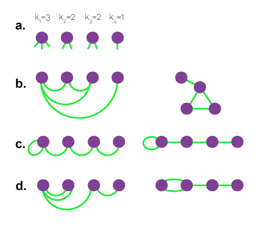
Image 4.15
The Configuration Model
The configuration model builds a network whose nodes have pre-defined degrees [40, 41]. The algorithm consists of the following steps:
Assign a degree to each node, represented as stubs or half-links. The degree sequence is either generated analytically from a preselected pk distribution (BOX 4.7), or it is extracted from the adjacency matrix of a real network. We must start from an even number of stubs, otherwise we are left with unpaired stubs.
Randomly select a stub pair and connect them. Then randomly choose another pair from the remaining 2L - 2 stubs and connect them. This procedure is repeated until all stubs are paired up. Depending on the order in which the stubs were chosen, we obtain different networks. Some networks include cycles (b), others self-loops (c) or multi-links (d). Yet, the expected number of self-loops and multi-links goes to zero in the N → ∞ limit.
Configuration Model
The configuration model, described in Image 4.15, helps us build a network with a pre-defined degree sequence. In the network generated by the model each node has a pre-defined degree ki, but otherwise the network is wired randomly. Consequently the network is often called a random network with a pre-defined degree sequence. By repeatedly applying this procedure to the same degree sequence we can generate different networks with the same pk (Image 4.15b-d). There are a couple of caveats to consider:
The probability to have a link between nodes of degree ki and kj is
Indeed, a stub starting from node i can connect to 2L - 1 other stubs. Of these, kj are attached to node j. So the probability that a particular stub is connected to a stub of node j is kj /(2L - 1). As node i has ki stubs, it has kj attempts to link to j, resulting in (4.24).
The obtained network contains self-loops and multi-links, as there is nothing in the algorithm to forbid a node connecting to itself, or to generate multiple links between two nodes. We can choose to reject stub pairs that lead to these, but if we do so, we may not be able to complete the network. Rejecting self-loops or multi-links also means that not all possible matchings appear with equal probability. Hence (4.24) will not be valid, making analytical calculations difficult. Yet, the number of self-loops and multi-links remain negligible, as the number of choices to connect to increases with N, so typically we do not need to exclude them [42].
The configuration model is frequently used in calculations, as (4.24) and its inherently random character helps us analytically calculate numerous network measures.
Degree-Preserving Randomization
As we explore the properties of a real network, we often need to ask if a certain network property is predicted by its degree distribution alone, or if it represents some additional property not contained in pk. To answer this question we need to generate networks that are wired randomly, but whose pk is identical to the original network. This can be achieved through degree-preserving randomization [43] described in Image 4.17b. The idea behind the algorithm is simple: We randomly select two links and swap them, if the swap does not lead to multi-links. Hence the degree of each of the four involved nodes in the swap remains unchanged. Consequently, hubs stay hubs and small-degree nodes retain their small degree, but the wiring diagram of the generated network is randomized. Note that degree-preserving randomization is different from full randomization, where we swap links without preserving the node degrees (Image 4.17a). Full randomization turns any network into an Erdős-Rényi network with a Poisson degree distribution that is independent of the original pk.
Image 4.17
Degree Preserving Randomization
Two algorithms can generate a randomized version of a given network [43], with different outcomes.
Full Randomization
This algorithm generates a random (Erdős–Rényi) network with the same N and L as the original network. We select randomly a source node (S1) and two target nodes, where the first target (T1) is linked directly to the source node and the second target (T2) is not. We rewire the S1-T1 link, turning it into an S1-T2 link. As a result the degree of the target nodes T1 and T2 changes. We perform this procedure once for each link in the network.
Degree-Preserving Randomization
This algorithm generates a network in which each node has exactly the same degree as in the original network, but the network’s wiring diagram has been randomized. We select two source (S1, S2) and two target nodes (T1, T2), such that initially there is a link between S1 and T1, and a link between S2 and T2. We then swap the two links, creating an S1-T2 and an S2-T1 link. The swap leaves the degree of each node unchanged.We repeat this procedure until we rewire each link at least once. Bottom Panels: Starting from a scale-free network (middle), full randomization eliminates the hubs and turns the network into a random network (left). In contrast, degree-preserving randomization leaves the hubs in place and the network remains scale-free (right).
Hidden Parameter Model
The configuration model generates self-loops and multi-links, features that are absent in many real networks. We can use the hidden parameter model (Image 4.18) to generate networks with a pre-defined pk but without multi-links and self-loops [44, 45, 46].
We start from N isolated nodes and assign each node i a hidden parameter ηi, chosen from a distribution ρ(η). The nature of the generated network depends on the selection of the {ηi} hidden parameter sequence. There are two ways to generate the appropriate hidden parameters:
ηi can be a sequence of N random numbers chosen from a pre-defined ρ(η) distribution. The degree distribution of the obtained network is
ηi can come from a deterministic sequence {η1, η2, ..., ηN}. The degree distribution of the obtained network is
The hidden parameter model offers a particularly simple method to generate a scale-free network. Indeed, using
as the sequence of hidden parameters, according to (4.27) the obtained network will have the degree distribution
for large k. Hence by choosing the appropriate α we can tune γ=1+1/α. We can also use 〈η〉 to tune 〈k〉 as (4.26) and (4.27) imply that 〈k〉 = 〈η〉.
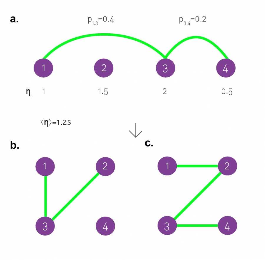
Image 4.18
Hidden Parameter Model
We start with N isolated nodes and assign to each node a hidden parameter ηi, which is either selected from a ρ(η) distribution or it is provided by a sequence {ηi}. We connect each node pair with probability
The figure shows the probability to connect nodes (1,3) and (3,4).
After connecting the nodes, we obtain the networks shown in (b) or (c), representing two independent realizations generated by the same hidden parameter sequence (a).
The expected number of links in the network generated by the model is
Similar to the random network model, L will vary from network to network, following an exponentially bounded distribution. If we wish to control the average degree 〈k〉 we can add L links to the network one by one. The end points i and j of each link are then chosen randomly with a probability proportional to ηi and ηj. In this case we connect i and j only if they were not connected previously.
In summary, the configuration model, degree-preserving randomization and the hidden parameter model can generate networks with a pre-defined degree distribution and help us analytically calculate key network characteristics. We will turn to these algorithms each time we explore whether a certain network property is a consequence of the network’s degree distribution, or if it represents some emergent property (BOX 4.8). As we use these algorithms, we must be aware of their limitations:
The algorithms do not tell us why a network has a certain degree distribution. Understanding the origin of the observed pk will be the subject of CHAPTERS 6 and 7.
Several important network characteristics, from clustering (CHAPTER 9) to degree correlations (CHAPTER 7), are lost during randomization.
Hence, the networks generated by these algorithms are a bit like a photograph of a painting: at first look they appear to be the same as the original. Upon closer inspection we realize, however, that many details, from the texture of the canvas to the brush strokes, are lost.
The three algorithms discussed above raise the following question: How do we decide which one to use? Our choice depends on whether we start from a degree sequence {ki} or a degree distribution pk and whether we can tolerate self-loops and multi-links between two nodes. The decision tree involved in this choice is provided in Image 4.20.
Image 4.20
Choosing a Generative Algorithm
The choice of the appropriate generative algorithm depends on several factors. If we start from a real network or a known degree sequence, we can use degree-preserving randomization, which guarantees that the obtained networks are simple and have the degree sequence of the original network. The model allows us to forbid multi-links or selfloops, while maintaining the degree sequence of the original network.
If we wish to generate a network with given pre-defined degree distribution pk, we have two options. If pk is known, the configuration model offers a convenient algorithm for network generation. For example, the model allows us generate a networks with a pure power law degree distribution pk=Ck–γ for k≥ kmin.
However, tuning the average degree 〈k〉 of a scale-free network within the configuration model is a tedious task, because the only available free parameter is kmin. Therefore, if we wish to alter 〈k〉, it is more convenient to use the hidden parameter model with parameter sequence (4.28). This way the tail of the degree distribution follows ~k-γ and by changing the number of links L we can to control 〈k〉.
Section 4.9
Summary
The scale-free property has played an important role in the development of network science for two main reasons:
Many networks of scientific and practical interest, from the WWW to the subcellular networks, are scale-free. This universality made the scale-free property an unavoidable issue in many disciplines.
Once the hubs are present, they fundamentally change the system’s behavior. The ultra-small property offers a first hint of their impact on a network’s properties; we will encounter many more examples in the coming chapters.
As we continue to explore the consequences of the scale-free property, we must keep in mind that the power-law form (4.1) is rarely seen in this pure form in real systems. The reason is that a host of processes affect the topology of each network, which also influence the shape of the degree distribution. We will discuss these processes in the coming chapters. The diversity of these processes and the complexity of the resulting pk confuses those who approach these networks through the narrow perspective of the quality of fit to a pure power law. Instead the scale-free property tells us that we must distinguish two rather different classes of networks:
Exponentially Bounded Networks
We call a network exponentially bounded if its degree distribution decrease exponentially or faster for high k. As a consequence ‹k2› is smaller than ‹k›, implying that we lack significant degree variations. Examples of pk in this class include the Poisson, Gaussian, or the simple exponential distribution (Table 4.2). Erdős-Rényi and Watts-Strogatz networks are the best known models network belonging to this class. Exponentially bounded networks lack outliers, consequently most nodes have comparable degrees. Real networks in this class include highway networks and the power grid.
Fat Tailed Networks
We call a network fat tailed if its degree distribution has a power law tail in the high-k region. As a consequence ‹k2› is much larger than ‹k›, resulting in considerable degree variations. Scale-free networks with a power-law degree distribution (4.1) offer the best known example of networks belonging to this class. Outliers, or exceptionally high-degree nodes, are not only allowed but are expected in these networks. Networks in this class include the WWW, the Internet, protein interaction networks, and most social and online networks.
While it would be desirable to statistically validate the precise form of the degree distribution, often it is sufficient to decide if a given network has an exponentially bounded or a fat tailed degree distribution (see ADVANCED TOPICS 4.A). If the degree distribution is exponentially bounded, the random network model offers a reasonable starting point to understand its topology. If the degree distribution is fat tailed, a scale-free network offers a better approximation. We will also see in the coming chapters that the key signature of the fat tailed behavior is the magniture of 〈k2〉: If 〈k2〉 is large, systems behave like scale-free networks; if 〈k2〉 is small, being comparable to 〈k〉(〈t〉+1), systems are well approximated by random networks.
In summary, to understand the properties of real networks, it is often sufficient to remember that in scale-free networks a few highly connected hubs coexist with a large number of small nodes. The presence of these hubs plays an important role in the system’s behavior. In this chapter we explored the basic characteristics of scale-free networks. We are left, therefore, with an important question: Why are so many real networks scale-free? The next chapter provides the answer.
Section 4.10
Homework
Hubs
Calculate the expected maximum degree kmax for the undirected networks listed in Table 4.1.
Friendship Paradox
The degree distribution pk expresses the probability that a randomly selected node has k neighbors. However, if we randomly select a link, the probability that a node at one of its ends has degree k is qk = Akpk, where A is a normalization factor.
Find the normalization factor A, assuming that the network has a power law degree distribution with 2 < γ < 3, with minimum degree kmin and maximum degree kmax.
In the configuration model qk is also the probability that a randomly chosen node has a neighbor with degree k. What is the average degree of the neighbors of a randomly chosen node?
Calculate the average degree of the neighbors of a randomly chosen node in a network with N = 104, γ= 2.3, kmin= 1 and kmax= 1, 000. Compare the result with the average degree of the network, 〈k〉.
How can you explain the "paradox" of (c), that is a node's friends have more friends than the node itself?
Generating Scale-Free Networks
Write a computer code to generate networks of size N with a power-law degree distribution with degree exponent γ. Refer to SECTION 4.9 for the procedure. Generate three networks with γ = 2.2 and with N = 103, N = 104 and N = 105 nodes, respectively. What is the percentage of multi-link and selfloops in each network? Generate more networks to plot this percentage in function of N. Do the same for networks with γ = 3.
Mastering Distributions
Use a software which includes a statistics package, like Matlab, Mathematica or Numpy in Python, to generate three synthetic datasets, each containing 10,000 integers that follow a power-law distribution with γ = 2.2, γ = 2.5 and γ = 3. Use kmin = 1. Apply the techniques described in ADVANCED TOPICS 4.C to fit the three distributions.
Section 4.11
Advanced Topic 3.A Power Laws
Power laws have a convoluted history in natural and social sciences, being interchangeably (and occasionally incorrectly) called fat-tailed, heavytailed, long-tailed, Pareto, or Bradford distributions. They also have a series of close relatives, like log-normal, Weibull, or Lévy distributions. In this section we discuss some of the most frequently encountered distributions in network science and their relationship to power laws.
Exponentially Bounded Distributions
Many quantities in nature, from the height of humans to the probability of being in a car accident, follow bounded distributions. A common property of these is that px decays either exponentially (e-x), or faster than exponentially (e-x2/σ2) for high x. Consequently the largest expected x is bounded by some upper value xmax that is not too different from 〈x〉. Indeed, the expected largest x obtained after we draw N numbers from a bounded px grows as xmax ~ logN or slower. This means that outliers, representing unusually high x-values, are rare. They are so rare that they are effectively forbidden, meaning that they do not occur with any meaningful probability. Instead, most events drawn from a bounded distribution are in the vicinity of 〈x〉.
The high-x regime is called the tail of a distribution. Given the absence of numerous events in the tail, these distributions are also called thin tailed.
Analytically the simplest bounded distribution is the exponential distribution e-λx. Within network science the most frequently encountered bounded distribution is the Poisson distribution (or its parent, the binomial distribution), which describes the degree distribution of a random network. Outside network science the most frequently encountered member of this class is the normal (Gaussian) distribution (Table 4.2).
Fat Tailed Distributions
The terms fat tailed, heavy tailed, or long tailed refer to px whose decay at large x is slower than exponential. In these distributions we often encounter events characterized by very large x values, usually called outliers or rare events. The power-law distribution (4.1) represents the best known example of a fat tailed distribution. An instantly recognizable feature of an fat tailed distribution is that the magnitude of the events x drawn from it can span several orders of magnitude. Indeed, in these distributions the size of the largest event after N trials scales as xmax ~ Nζ where ζ is determined by the exponent γ characterizing the tail of the px distribution. As Nζ grows fast, rare events or outliers occur with a noticeable frequency, often dominating the properties of the system.
The relevance of fat tailed distributions to networks is provided by several factors:
Many quantities occurring in network science, like degrees, link weights and betweenness centrality, follow a power-law distribution in both real and model networks.
The power-law form is analytically predicted by appropriate network models (CHAPTER 5).
Crossover Distribution (Log-Normal, Stretched Exponential)
When an empirically observed distribution appears to be between a power law and exponential, crossover distributions are often used to fit the data. These distributions may be exponentially bounded (power law with exponential cutoff), or not bounded but decay faster than a power law (log-normal or stretched exponential). Next we discuss the properties of several frequently encountered crossover distributions.
Power law with exponential cut-off is often used to fit the degree distribution of real networks. Its density function has the form:
where x > 0 and γ > 0 and Γ(s,y) denotes the upper incomplete gamma function. The analytical form (4.30) directly captures its crossover nature: it combines a power-law term, a key component of fat tailed distributions, with an exponential term, responsible for its exponentially bounded tail. To highlight its crossover characteristics we take the logarithm of (4.30),
For x ≪ 1/λ the second term on the r.h.s dominates, suggesting that the distribution follows a power law with exponent γ. Once x ≫ 1/λ, the λx term overcomes the ln x term, resulting in an exponential cutoff for high x.
Stretched exponential (Weibull distribution) is formally similar to (4.30) except that there is a fractional power law in the exponential. Its name comes from the fact that its cumulative distribution function is one minus a stretched exponential function P(x) = e-(λx)β (4.32) which leads to density function
In most applications x varies between 0 and +∞. In (4.32) β is the stretching exponent, determining the properties of p(x):
For β = 1 we recover a simple exponential function.
If β is between 0 and 1, the graph of log p(x) versus x is “stretched”, meaning that it spans several orders of magnitude in x. This is the regime where a stretched exponential is difficult to distinguish from a pure power law. The closer β is to 0, the more similar is p(x) to the power law x-1.
If β > 1 we have a “compressed” exponential function, meaning that x varies in a very narrow range.
For β = 2 (4.33) reduces to the Rayleigh distribution.
As we will see in CHAPTERS 5 and 6, several network models predict a streched exponential degree distribution.
A log-normal distribution (Galton or Gibrat distribution) emerges if ln x follows a normal distribution. Typically a variable follows a log-normal distribution if it is the product of many independent positive random numbers. We encounter log-normal distributions in finance, representing the compound return from a sequence of trades.
The probability density function of a log-normal distribution is
Hence a log-normal is like a normal distribution except that its variable in the exponential term is not x, but ln x.
To understand why a log-normal is occasionally used to fit a power law distribution, we note that
captures the typical variation of the order of magnitude of x. Therefore now ln x follows a normal distribution, which means that x can vary rather widely. Depending on the value of σ the log-normal distribution may resemble a power law for several orders of magnitude. This is also illustrated in Table 4.2, that shows that 〈x2〉 grows exponentially with σ, hence it can be very large.
In summary, in most areas where we encounter fat-tailed distributions, there is an ongoing debate asking which distribution offers the best fit to the data. Frequently encountered candidates include a power law, a stretched exponential, or a log-normal function. In many systems empirical data is not sufficient to distinguish these distributions. Hence as long as there is empirical data to be fitted, the debate surrounding the best fit will never die out.
The debate is resolved by accurate mechanistic models, which analytically predict the expected degree distribution.We will see in the coming chapters that in the context of networks the models predict Poisson, simple exponential, stretched exponential, and power law distributions. The remaining distributions in Table 4.2 are occasionally used to fit the degrees of some networks, despite the fact that we lack theoretical basis for their relevance for networks.
NAME
Poisson (discrete)
Exponential (discrete)
Exponential (continuous)
Power law (discrete)
Power law (continuous)
Power law with cutoff (continuous)
Stretched exponential (continuous)
Log-normal (continuous)
Normal (continuous)
Table 4.2
Distributions in Network Science
The table lists frequently encountered distributions in network science. For each distribution we show the density function px, the appropriate normalization constant C such that
for the continuous case or
for the discrete case. Given that 〈x〉 and 〈x2〉 play an important role in network theory, we show the analytical form of these two quantities for each distribution. As some of these distributions diverge at x = 0, for most of them 〈x〉 and 〈x2〉 are calculated assuming that there is a small cutoff xmin in the system. In networks xmin often corresponds to the smallest degree, kmin, or the smallest degree for which the appropriate distribution offers a good fit.
Image 4.21
Distributions Visualized
Linear and the log-log plots for the most frequently encountered distributions in network science. For definitions see Table 4.2
Plotting the degree distribution is an integral part of analyzing the properties of a network. The process starts with obtaining Nk, the number of nodes with degree k. This can be provided by direct measurement or by a model. From Nk we calculate pk = Nk /N. The question is, how to plot pk to best extract its properties.
Use a Log-Log Plot
In a scale-free network numerous nodes with one or two links coexist with a few hubs, representing nodes with thousands or even millions of links. Using a linear k-axis compresses the numerous small degree nodes in the small-k region, rendering them invisible. Similarly, as there can be orders of magnitude differences in pk for k = 1 and for large k, if we plot pk on a linear vertical axis, its value for large k will appear to be zero (Image 4.22a). The use of a log-log plot avoids these problems. We can either use logarithmic axes, with powers of 10 (used throughout this book, Image 4.22b) or we can plot log pk in function of log k (equally correct, but slightly harder to read). Note that points with pk =0 or k=0 are not shown on a log-log plot as log 0=-∞.
Avoid Linear Binning
The most flawed method (yet frequently seen in the literature) is to simply plot pk = Nk/N on a log-log plot (Image 4.22b). This is called linear binning, as each bin has the same size Δk = 1. For a scale-free network linear binning results in an instantly recognizable plateau at large k, consisting of numerous data points that form a horizontal line (Image 4.22b). This plateau has a simple explanation: Typically we have only one copy of each high degree node, hence in the high-k region we either have Nk=0 (no node with degree k) or Nk=1 (a single node with degree k). Consequently linear binning will either provide pk=0, not shown on a log-log plot, or pk = 1/N, which applies to all hubs, generating a plateau at pk = 1/N.
This plateau affects our ability to estimate the degree exponent γ. For example, if we attempt to fit a power law to the data shown in Image 4.22b using linear binning, the obtained γ is quite different from the real value γ=2.5. The reason is that under linear binning we have a large number of nodes in small k bins, allowing us to confidently fit pk in this regime. In the large-k bins we have too few nodes for a proper statistical estimate of pk. Instead the emerging plateau biases our fit. Yet, it is precisely this high-k regime that plays a key role in determining γ. Increasing the bin size will not solve this problem. It is therefore recommended to avoid linear binning for fat tailed distributions.
Image 4.22
Plotting a Degree Distributions
A degree distribution of the form pk ~ (k + k0)-γ, with k0=10 and γ=2.5, plotted using the four procedures described in the text:
Linear Scale, Linear Binning.
It is impossible to see the distribution on a lin-lin scale. This is the reason why we always use log-log plot for scale-free networks.
Log-Log Scale, Linear Binning.
Now the tail of the distribution is visible but there is a plateau in the high-k regime, a consequence of linear binning.
Log-Log Scale, Log-Binning.
With log-binning the plateau dissappears and the scaling extends into the high-k regime. For reference we show as light grey the data of (b) with linear binning.
Log-Log Scale, Cumulative.
The cumulative degree distribution shown on a log-log plot.
Use Logarithmic Binning
Logarithmic binning corrects the non-uniform sampling of linear binning. For log-binning we let the bin sizes increase with the degree, making sure that each bin has a comparable number of nodes. For example, we can choose the bin sizes to be multiples of 2, so that the first bin has size b0=1, containing all nodes with k=1; the second has size b1=2, containing nodes with degrees k=2, 3; the third bin has size b2=4 containing nodes with degrees k=4, 5, 6, 7. By induction the nth bin has size 2n-1 and contains all nodes with degrees k=2n-1, 2n-1+1, ..., 2n-1-1. Note that the bin size can increase with arbitrary increments, bn= cn, where c > 1. The degree distribution is given by p〈kn〉=Nn/bn, where Nn is the number of nodes found in the bin n of size bn and 〈kn〉 is the average degree of the nodes in bin bn.
The logarithmically binned pk is shown in Image 4.22c. Note that now the scaling extends into the high-k plateau, invisible under linear binning. Therefore logarithmic binning extracts useful information from the rare high degree nodes as well (BOX 4.10).
Use Cumulative Distribution
Another way to extract information from the tail of pk is to plot the complementary cumulative distribution
which again enhances the statistical significance the high-degree region. If pk follows the power law (4.1), then the cumulative distribution scales as
The cumulative distribution again eliminates the plateau observed for linear binning and leads to an extended scaling region (Image 4.22d), allowing for a more accurate estimate of the degree exponent.
In summary, plotting the degree distribution to extract its features requires special attention. Mastering the appropriate tools can help us better explore the properties of real networks (BOX 4.10).
Section 4.13
Advanced Topic 3.C Estimating the Degree Exponent
As the properties of scale-free networks depend on the degree exponent (SECTION 4.7), we need to determine the value of γ. We face several difficulties, however, when we try to fit a power law to real data. The most important is the fact that the scaling is rarely valid for the full range of the degree distribution. Rather we observe small- and high- degree cutoffs (BOX 4.10), denoted in this section with Kmin and Kmax, within which we have a clear scaling region. Note that Kmin and Kmax are different from Kmin and Kmax, the latter corresponding to the smallest and largest degrees in a network. They can be the same as ksat and kcut discussed in BOX 4.10. Here we focus on estimating the small degree cutoff Kmin, as the high degree cutoff can be determined in a similar fashion. The reader is advised to consult the discussion on systematic problems provided at the end of this section before implementing this procedure.
Online Resource 4.2 Fitting power-law
The algorithmic tools to perform the fitting procedure described in this section are available at http://tuvalu.santafe.edu/~aaronc/powerlaws/.
Fitting Procedure
As the degree distribution is typically provided as a list of positive integers kmin , ..., kmax, we aim to estimate γ from a discrete set of data points [47]. We use the citation network to illustrate the procedure. The network consists of N=384,362 nodes, each node representing a research paper published between 1890 and 2009 in journals published by the American Physical Society. The network has L = 2,353,984 links, each representing a citation from a published research paper to some other publication in the dataset (outside citations are ignored). For no particular reason, this is not the citation dataset listed in Table 4.1. See [48] for an overall characterization of this data. The steps of the fitting process are [47]:
Choose a value of Kmin between kmin and kmax. Estimate the value of the degree exponent corresponding to this Kmin using
With the obtained (γ, Kmin) parameter pair assume that the degree distribution has the form
hence the associated cumulative distribution function (CDF) is
Use the Kormogorov-Smirnov test to determine the maximum distance D between the CDF of the data S(k) and the fitted model provided by (4.43) with the selected (γ, kmin) parameter pair,
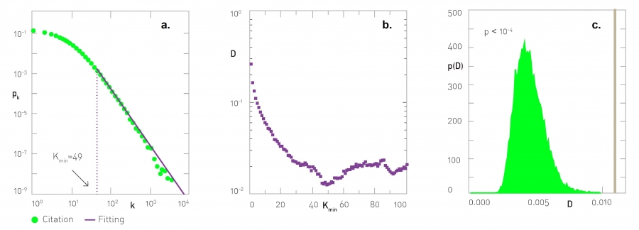
Repeat steps (1-3) by scanning the whole Kmin range from kmin to kmax. We aim to identify the Kmin value for which D provided by (4.44) is minimal. To illustrate the procedure, we plot D as a function of Kmin for the citation network (Image 4.24b). The plot indicates that D is minimal for Kmin= 49, and the corresponding γ estimated by (4.41), representing the optimal fit, is γ=2.79. The standard error for the obtained degree exponent is
which implies that the best fit is γ ± σγ. For the citation network we obtain σγ=0.003, hence γ=2.79(3).
Note that in order to estimate γ datasets smaller than N=50 should be treated with caution.
Image 4.24
Maximum Likelihood Estimation
The degree distribution pk of the citation network, where the straight purple line represents the best fit based on the model (4.39).
The values of Kormogorov-Smirnov test vs. Kmin for the citation network.
p(Dsynthetic) for M=10,000 synthetic datasets, where the grey line corresponds to the Dreal value extracted for the citation network.
Goodness-of-fit
Just because we obtained a (γ, Kmin) pair that represents an optimal fit to our dataset, does not mean that the power law itself is a good model for the studied distribution.We therefore need to use a goodness-of-fit test, which generates a p-value that quantifies the plausibility of the power law hypothesis. The most often used procedure consists of the following steps:
Use the cumulative distribution (4.43) to estimate the KS distance between the real data and the best fit, that we denote by Dreal. This is step 3 above, taking the value of D for Kmin that offered the best fit to the data. For the citation data we obtain Dreal = 0.01158 for Kmin=49 (Image 4.24c).
Use (4.42) to generate a degree sequence of N degrees (i.e. the same number of random numbers as the number of nodes in the original dataset) and substitute the obtained degree sequence for the empirical data, determining Dsynthetic for this hypothetical degree sequence. Hence Dsynthetic represents the distance between a synthetically generated degree sequence, consistent with our degree distribution, and the real data.
The goal is to see if the obtained Dsynthetic is comparable to Dreal. For this we repeat step (2) M times (M ≫ 1), and each time we generate a new degree sequence and determine the corresponding Dsynthetic, eventually obtaining the p(Dsynthetic) distribution. Plot p(Dsynthetic) and show as a vertical bar Dreal (Image 4.24c). If Dreal is within the p(Dsynthetic) distribution, it means that the distance between the model providing the best fit and the empirical data is comparable with the distance expected from random degree samples chosen from the best fit distribution. Hence the power law is a reasonable model for the data. If, however, Dreal falls outside the p(Dsynthetic) distribution, then the power law is not a good model - some other function is expected to describe the original pk better.
While the distribution shown in Image 4.24c may be in some cases useful to illustrate the statistical significance of the fit, in general it is better to assign a p-number to the fit, given by
The closer p is to 1, the more likely that the difference between the empirical data and the model can be attributed to statistical fluctuations alone. If p is very small, the model is not a plausible fit to the data.
Typically, the model is accepted if p > 1%. For the citation network we obtain p < 10-4, indicating that a pure power law is not a suitable model for the original degree distribution. This outcome is somewhat surprising, as the power-law nature of citation data has been documented repeatedly since 1960s [7, 8]. This failure indicates the limitation of the blind fitting to a power law, without an analytical understanding of the underlying distribution.
Fitting Real Distributions
To correct the problem, we note that the fitting model (4.44) eliminates all the data points with k < Kmin. As the citation network is fat tailed, choosing Kmin = 49 forces us to discard over 96% of the data points. Yet, there is statistically useful information in the k < Kmin regime, that is ignored by the previous fit. We must introduce an alternate model that resolves this problem.
As we discussed in BOX 4.10, the degree distribution of many real networks, like the citation network, does not follow a pure power law. It often has low degree saturations and high degree cutoffs, described by the form
and the associated CDF is
where ksat and kcut correspond to low-k saturation and the large-k cutoff, respectively. The difference between our earlier procedure and (4.47) is that we now do not discard the points that deviate from a pure power law, but instead use a function that offers a better fit to the whole degree distribution, from kmin to kmax.
Our goal is to find the fitting parameters ksat, kcut, and γ of the model (4.47), which we achieve through the following steps (Image 4.25):
Pick a value for ksat and kcut between Kmin and Kmax. Estimate the value of the degree exponent γ using the steepest descend method that maximizes the log-likelihood function
That is, for fixed (ksat, kcut) we vary γ until we find the maximum of (4.49).
With the obtained γ(ksat, kcut) assume that the degree distribution has the form (4.47). Calculate the Kormogorov Smirnov parameter D between the cumulative degree distribution (CDF) of the original data and the fitted model provided by (4.47).
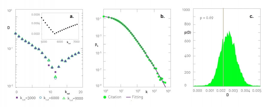
Change ksat and kcut, and repeat steps (1-3), scanning with ksat from kmin= 0 to kmax and scanning with kcut from kmin= k0 to kmax. The goal is to identify ksat and kcut values for which D is minimal. We illustrate this by plotting D in function of ksat for several kcut values in Image 4.25a for our citation network. The (ksat, kcut) for which D is minimal, and the corresponding γ is provided by (4.41), represent the optimal parameters of the fit. For our dataset the optimal fit is obtained for /ksat= 12 and kcut= 5,691, providing the degree exponent γ= 3.028. We find that now D for the real data is within the generated p(D) distribution (Image 4.25c), and the associated p-value is 69%.
Image 4.25
Estimating the Scaling Parameters for Citation Networks
The Kormogorov-Smirnov parameter D vs. ksat for kcat = 3,000, 6,000, 9,000, respectively. The curve indicates that ksat= 12 corresponds to the minimal D. Inset: D vs. kcut for ksat= 12, indicating that kcut =5,691 minimizes D
Degree distribution pk where the straight line represents the best estimate from (a). Now the fit accurately captures the whole curve, not only its tail, or it did in Image 4.24a.
p(Dsynthetic) for M = 10,000 synthetic datasets. The grey line corresponds to the Dreal value from the citation network.
Systematic Fitting Issues
The procedure described above may offer the impression that determining the degree exponent is a cumbersome but straightforward process. In reality these fitting methods have some well known limitations:
A pure power law is an idealized distribution that emerges in its form (4.1) only in simple models (CHAPTER 5). In reality, a whole range of processes contribute to the topology of real networks, affecting the precise shape of the degree distribution. These processes will be discussed in CHAPTER 6. If pk does not follow a pure power law, the methods described above, designed to fit a power law to the data, will inevitably fail to detect statistical significance. While this finding can mean that the network is not scale-free, it most often means that we have not yet gained a proper understanding of the precise form of the degree distribution. Hence we are fitting the wrong functional form of pk to the dataset.
The statistical tools used above to test the goodness-of-fit rely on the Kolmogorov-Smirnov criteria, which measures the maximum distance between the fitted model and the dataset. If almost all data points follow a perfect power law, but a single point for some reason deviates from the curve, we will loose the fit’s statistical significance. In real systems there are numerous reasons for such local deviations that have little impact on the system’s overall behavior. Yet, removing these “outliers” could be seen as data manipulation; if kept, however, one cannot detect the statistical significance of the power law fit.
A good example is provided by the actor network, whose degree distribution follows a power law for most degrees. There is, however, a prominent outlier at k = 1,287, thanks to the 1956 movie Around the World in Eighty Days. This is the only movie where imdb.com the source of the actor network, lists all the normally uncredited extras in the cast. Hence the movie appears to have 1,288 actors. The second largest movie in the dataset has only 340 actors. Since each extra has links only to the 1,287 extras that played in the same movie, we have a local peak in pk at k=1,287. Thanks to this peak, the degree distribution, fitted to a power law, fails to pass the Kolmogorov-Smirnov criteria. Indeed, as indicated in Table 4.3, neither the pure power law fit, nor a power law with high-degree cutoff offers a statistically significant fit. Yet, ultimately this single point does not alter the power law nature of the degreee distribution.
As a result of the issues discussed above, the methodology described to fit a power law distribution often predicts a small scaling regime, forcing us to remove a huge fraction of the nodes (often as many as 99%, see Table 4.4) to obtain a statistically significant fit. Once plotted next to the original dataset, the obtained fit can be at times ridiculous, even if the method predits statistical significance.
λ
kmin
P-VALUE
PERCENTAGE
Power Grid
0.517
4
0.91
12%
Table 4.3
Degree Fluctuations in Real Networks
For the power grid a power law degree distribution does not offer a statistically significant fit. Indeed, we will encounter numerous evidence that the underlying network is not scale-free. We used the fitting procedure described in this section to fit the exponential function e-λk to the degree distribution of the power grid, obtaining a statistically significant fit. The table shows the obtained λ parameters, the kmin over which the fit is valid, the obtained p-value, and the percentage of data points included in the fit.
In summary, estimating the degree exponent is still not yet an exact science. We continue to lack methods that would estimate the statistical significance in a manner that would be acceptable to a practitioner. The blind application of the tools describe above often leads to either fits that obviously do not capture the trends in the data, or to a false rejection of the power-law hypothesis. An important improvement is our ability to derive the expected form of the degree distribution, a problem discussed in CHAPTER 6.
K-γ; [Kmin, ∞]
(k+ksat)-γe-k/kcut
γ
Kmin
P-VALUE
PERCENT
γ
kset
kcut
P-VALUE
Internet
3.42
72
0.13
0.6%
3.55
8
8500
0.00
WWW (IN)
2.00
1
0.00
100%
1.97
0
660
0.00
WWW (OUT)
2.31
7
0.00
15%
2.82
8
8500
0.00
Power Grid
4.00
5
0.00
12%
8.56
19
14
0.00
Mobile Phone Calls (in)
4.69
9
0.34
2.6%
6.95
15
10
0.00
Mobile Phone Calls (out)
5.01
11
0.77
1.7%
7.23
15
10
0.00
Email-Pre (in)
3.43
88
0.11
0.2%
2.27
0
8500
0.00
Email-Pre (out)
2.03
3
0.00
1.2%
2.55
0
8500
0.00
Science Collaboration
3.35
25
0.0001
5.4%
1.50
17
12
0.00
Actor Network
2.12
54
0.00
33%
-
-
-
0.00
Citation Network (in)
2.79
51
0.00
3.0%
3.03
12
5691
0.69
Citation Network (out)
4.00
19
0.00
14%
-0.16
5
10
0.00
E.Coli Metabolism (in)
2.43
3
0.00
57%
3.85
19
12
0.00
E.Coli Metabolism (out)
2.90
5
0.00
34%
2.56
15
10
0.00
Yeast Protein Interactions
2.89
7
0.67
8.3%
2.95
2
90
0.52
Table 4.4
Fitting Parameters for Real Networks
The estimated degree exponents and the appropriate fit parameters for the reference networks studied in this book. We implement two fitting strategies, the first aiming to fit a pure power law in the region (Kmin, ∞) and the second fits a power law with saturation and exponential cutoff to the whole dataset. In the table we show the obtained γ exponent and Kmin for the fit with the best statistical significance, the p-value for the best fit and the percentage of the data included in the fit. In the second case we again show the exponent γ, the two fit parameters, ksat and kcut, and the p-value of the obtained fit. Note that p > 0.01 is considered to be statistically significant.
Section 4.14
Bibliography
[1] H. Jeong, R.Albert, and A.-L. Barabási. Internet: Diameter of the world-wide web. Nature, 401:130-131, 1999.
[2] A.-L. Barabási and R.Albert. Emergence of scaling in random networks. Science, 286:509-512, 1999.
[3] V. Pareto. Cours d’Économie Politique: Nouvelle édition par G.- H. Bousquet et G. Busino, Librairie Droz, Geneva, 299–345, 1964.
[4] A.-L. Barabási. Linked: The New Science of Networks. Plume, New York, 2002.
[5] M. Faloutsos, P. Faloutsos, and C. Faloutsos. On power-law relationships of the internet topology. Proceedings of SIGCOMM. Comput. Commun. Rev. 29: 251-262, 1999.
[6] R. Pastor-Satorras and A.Vespignani. Evolution and Structure of the Internet: A Statistical Physics Approach. Cambridge University Press, Cambridge, 2004.
[7] D. J. De Solla Price. Networks of Scientific Papers. Science 149: 510- 515, 1965.
[8] S. Redner. How Popular is Your Paper? An Empirical Study of the Citation Distribution. Eur. Phys. J. B 4: 131, 1998.
[9] R. Kumar, P. Raghavan, S. Rajalopagan, and A.Tomkins. Extracting Large-Scale Knowledge Bases from the Web. Proceedings of the 25thVLDBConference, Edinburgh,Scotland,pp.639-650,1999.
[10] A.-L. Barabási, R.Albert, and H. Jeong. Mean-field theory of scalefree random networks. Physica A 272:173-187, 1999.
[11] H. Jeong, B. Tombor, R. Albert, Z. N. Oltvai, and A.-L. Barabási. The large-scale organization of metabolic networks. Nature 407: 651-654, 2000.
[12] A. Wagner, A. and D.A. Fell. The small world inside large metabolic networks. Proc. R. Soc. Lond. B 268: 1803–1810, 2001.
[13] W. Aiello, F. Chung, and L.A. Lu. Random graph model for massive graphs, Proc. 32nd ACM Symp. Theor. Comp, 2000.
[14] H. Jeong, B. Tombor, S. P. Mason, A.-L. Barabási, and Z.N. Oltvai. Lethality and centrality in protein networks. Nature 411: 41-42, 2001.
[15] A. Wagner. How the global structure of protein interaction networks evolves. Proc. R. Soc. Lond. B 270: 457–466, 2003.
[16] M. E. J. Newman. The structure of scientific collaboration networks. Proc. Natl.Acad. Sci. 98: 404-409, 2001.
[17] A.-L. Barabási, H. Jeong, E. Ravasz, Z. Néda, A. Schubert, and T. Vicsek. Evolution of the social network of scientific collaborations. Physica A 311: 590-614, 2002.
[18] F. Liljeros, C.R. Edling, L.A.N. Amaral, H.E. Stanley, and Y. Aberg. The Web of Human Sexual Contacts. Nature 411: 907-908, 2001.
[19] R. Ferrer i Cancho and R.V. Solé. The small world of human language. Proc. R. Soc. Lond. B 268: 2261-2265, 2001.
[20] R. Ferrer i Cancho, C. Janssen, and R.V. Solé. Topology of technology graphs: Small world patterns in electronic circuits. Phys. Rev. E 64: 046119, 2001.
[21] S. Valverde and R.V. Solé. Hierarchical Small Worlds in Software Architecture. arXiv:cond-mat/0307278, 2003.
[22] H. Ebel, L.-I. Mielsch, and S. Bornholdt. Scale-free topology of email networks. Phys. Rev. E 66: 035103(R), 2002.
[23] J.P.K. Doye. Network Topology of a Potential Energy Landscape: A Static Scale-Free Network. Phys. Rev. Lett. 88: 238701, 2002.
[24] J.-P. Onnela, J. Saramaki, J. Hyvonen, G. Szabó, D. Lazer, K. Kaski, J. Kertesz, and A.-L. Barabási. Structure and tie strengths in mobile communication networks. Proceedings of the National Academy of Sciences 104: 7332-7336 (2007).
[25] H. Kwak, C. Lee, H. Park, S. Moon. What is Twitter, a social network or a news media? Proceedings of the 19th international conference on World Wide Web, 591-600, 2010.
[26] M. Cha, H. Haddadi, F. Benevenuto and K. P. Gummadi. Measuring user influence in Twitter: The million follower fallacy. Proceedings of international AAAI Conference on Weblogs and Social, 2010.
[27] J. Ugander, B. Karrer, L. Backstrom, and C. Marlow. The Anatomy of the Facebook Social Graph. ArXiv:1111.4503, 2011.
[28] L.A.N. Amaral, A. Scala, M. Barthelemy and H.E. Stanley. Classes of small-world networks. Proceeding National Academy of Sciences U. S. A. 97:11149-11152, 2000.
[29] R. Cohen and S. Havlin. Scale free networks are ultrasmall. Phys. Rev. Lett. 90, 058701, 2003.
[30] B. Bollobás and O. Riordan. The Diameter of a Scale-Free Random Graph. Combinatorica, 24: 5-34, 2004.
[31] R. Cohen and S. Havlin. Complex Networks - Structure, Robustness and Function. Cambridge University Press, Cambridge, 2010.
[32] K.-I. Goh, B. Kahng, and D. Kim. Universal behavior of load distribution in scale-free networks. Phys. Rev. Lett. 87: 278701, 2001.
[33] F. Karinthy. Láncszemek, in Minden másképpen van. Budapest, Atheneum Irodai es Nyomdai R.-T. Kiadása, 85–90, 1929. English translation in: M.E.J. Newman, A.-L. Barabási, and D. J. Watts. The Structure and Dynamics of Networks. Princeton University Press, Princeton, 2006.
[34] P.S. Dodds, R. Muhamad and D.J. Watts. An experimental study to search in global social networks. Science 301: 827-829, 2003.
[35] P. Erdős and T. Gallai. Graphs with given degrees of vertices. Matematikai Lapok, 11:264-274, 1960.
[36] C.I. Del Genio, H. Kim, Z. Toroczkai, and K.E. Bassler. Efficient and exact sampling of simple graphs with given arbitrary degree sequence. PLoS ONE, 5: e10012, 04 2010.
[37] V. Havel. A remark on the existence of finite graphs. Casopis Pest. Mat., 80:477-480, 1955.
[38] S. Hakimi. On the realizability of a set of integers as degrees of the vertices of a graph. SIAM J.Appl. Math., 10:496-506, 1962.
[39] I. Charo Del Genio, G. Thilo, and K.E. Bassler. All scale-free networks are sparse. Phys. Rev. Lett. 107:178701, 10 2011.
[40] B. Bollobás. A probabilistic proof of an asymptotic formula for the number of labelled regular graphs. European J. Combin. 1: 311– 316, 1980.
[41] M. Molloy and B. A. Reed. Critical Point for Random Graphs with a Given Degree Sequence. Random Structures and Algorithms, 6: 161-180, 1995.
[42] M. Newman. Networks: An Introduction. Oxford University, Oxford, 2010.
[43] S. Maslov and K. Sneppen. Specificity and stability in topology of protein networks. Science, 296:910-913, 2002.
[44] G. Caldarelli, I. A. Capocci, P. De Los Rios, and M.A. Muñoz. Scale- Free Networks from Varying Vertex Intrinsic Fitness. Phys. Rev. Lett. 89: 258702, 2002.
[45] B. Söderberg. General formalism for inhomogeneous random graphs. Phys. Rev. E 66: 066121, 2002.
[46] M. Boguñá and R. Pastor-Satorras. Class of correlated random networks with hidden variables. Phys. Rev. E 68: 036112, 2003.
[47] A. Clauset, C.R. Shalizi, and M.E.J. Newman. Power-law distributions in empirical data. SIAM Review S1: 661-703, 2009.
[48] S. Redner. Citation statistics from 110 years of physical review. Physics Today, 58:49, 2005.